In this series of articles, I am going to focus on the basis of Deep Learning, and progressively move toward recent research papers and more advanced techniques. As I am particularly interested in computer vision, I will explore some examples applied to object detection or emotion recognition for example.

History of Deep Learning

Favio Vázquez has created a great summary of the deep learning timeline :

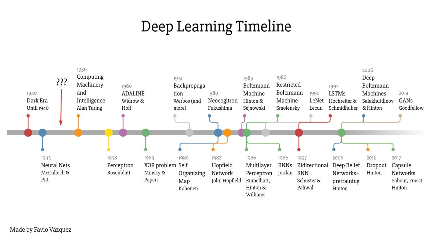
Among the most important events on this timeline, I would highlight :

1958: the Rosenblatt’s Perceptron
1974: Backpropagation
1985: Boltzmann Machines
1986: MLP, RNN
2012: Dropout
2014: GANs

Why neurons?

Neuronal networks have been at the core of the development of Deep Learning these past years. But what is the link between a neuron biologically speaking and a deep learning algorithm?

Neural networks are a set of algorithms that have been developed imitate the human brain in the way we identify patterns. In neurology, researchers study the way we process information. We have outstanding abilities to process information quickly and extract patterns.

Take a quick example: we can process information pre-attentively. Indeed, in less time than an eye blink (200ms), we can identify elements that pop out from an image. On the other hand, if the element does not pop out enough, we need to make a sequential search, which is much longer.

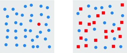
The information that we process in this example allows us to make a binary classification (major class vs the outlier we’re trying to identify). To understand what’s going on, I’ll make a brief introduction (to the extent of my limited knowledge in this field) to the architecture of a neuron biologically speaking.

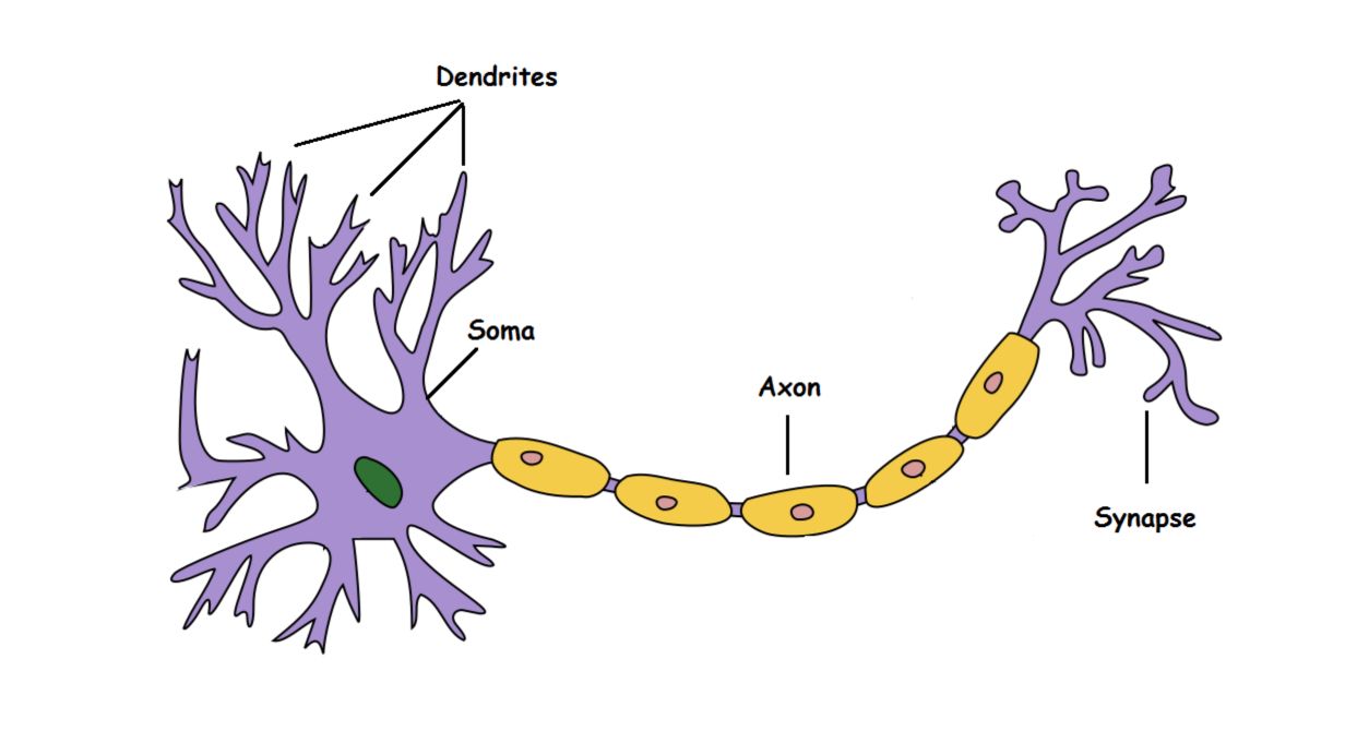
Here’s what the different components are made for :

Dendrite: Receives signals from other neurons
Soma: Processes the information
Axon: Transmits the output of a neuron
Synapse: Point of connection to other neurons

A neuron takes an input signal (dendrite), processes the information (soma) and passes the output to other connected neurons (axon to synapse to other neuron’s dendrite).

Now, this might be biologically inaccurate as there is a lot more going on out there but on a higher level, this is what is going on with a neuron in our brain — takes an input, processes it, throws out an output.

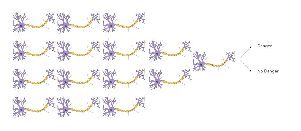
Suppose that you are walking on a crosswalk and want to determine whether there is a dangerous situation or not. The information to process might be :

visual, e.g. a car is close
audio, e.g. the sound of the car, a klaxon…

A series of neurons will process the information. Intrinsically, using both channels, you will :

determine how close the car is
and how fast the car is going

The neurons are activated depending on the given criteria. This will eventually lead to some sort of binary classification: Is there a danger or not? During the information processing, a large number of neurons will activate sequentially, and eventually lead to a single output.

This is an overly simplified representation, and I don’t have sufficient knowledge to expand this section.

The McCulloch-Pitts Neuron (1943)

The first computational model of a neuron was proposed by Warren McCulloch and Walter Pitts in 1943. We’ll cover this first simple model as an introduction to the Rosenblatt’s Perceptron.

How does the McCulloch-Pitts neuron work?

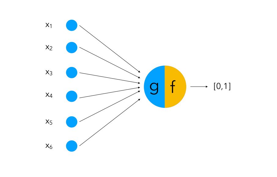
The first part is to process a series of boolean inputs (just like dendrites). If an input takes the value 1, we say that neuron fires.

We then process the information into an aggregative function g (can be compared to Soma) that performs a simple aggregation of the values of each input. Then, the function f compares the output of g to a threshold or a condition.

We can make several algorithms with this :

OR: the f function checks if the sum g is equal to 1
AND: the f function checks if the sum g is equal to the number of inputs
GREATER THAN: the f function checks if the sum g is equal to a threshold \(\theta\)

The simplest binary classification can be achieved the following way :

\(y = 1\) if \(\sum_i x_i ≥ 0\), else \(y = 0\)

There are however several limitations to McCulloch-Pitts Neurons :

it cannot process non-boolean inputs
it gives equal weights to each input
the threshold \(\theta\) much be chosen by hand
it implies a linearly separable underlying distribution of the data

For all these reasons, a necessary upgrade was required.

The Rosenblatt’s Perceptron (1957)

The classic model

The Rosenblatt’s Perceptron was designed to overcome most issues of the McCulloch-Pitts neuron :

it can process non-boolean inputs
and it can assign different weights to each input automatically
the threshold \(\theta\) is computed automatically

A perceptron is a single layer Neural Network. A perceptron can simply be seen as a set of inputs, that are weighted and to which we apply an activation function. This produces sort of a weighted sum of inputs, resulting in an output. This is typically used for classification problems, but can also be used for regression problems.

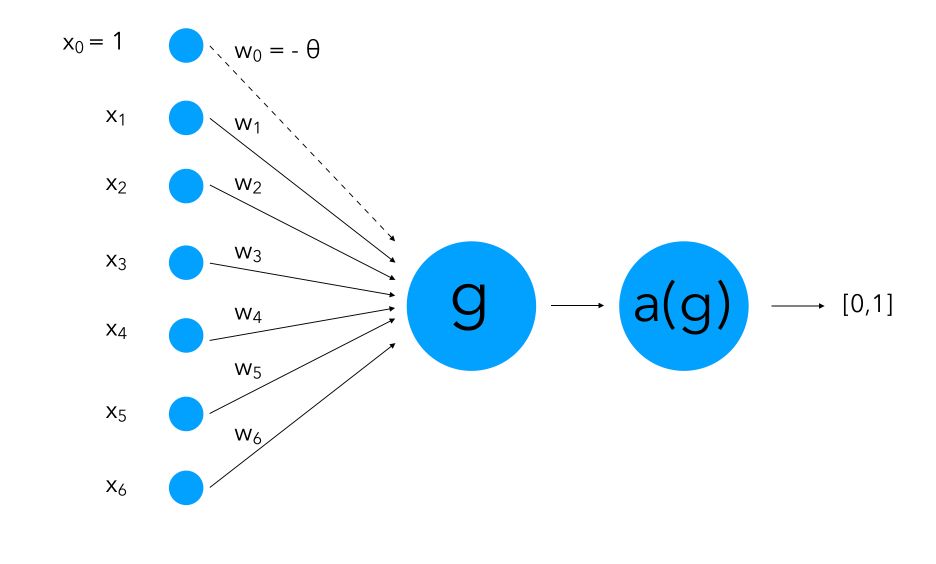
The perceptron was first introduced in 1957 by Franck Rosenblatt. Since then, it has been the core of Deep Learning. We can represent schematically a perceptron as :

We attach to each input a weight ( \(w_i\)) and notice how we add an input of value 1 with a weight of \(- \theta\). This is called bias. What we are doing is instead of having only the inputs and the weight and compare them to a threshold, we also learn the threshold as a weight for a standard input of value 1.

The inputs can be seen as neurons and will be called the input layer. Altogether, these neurons and the function (which we’ll cover in a minute) form a perceptron.

How do we make classification using a perceptron then?

\(y = 1\) if \(\sum_i w_i x_i ≥ 0\), else \(y = 0\)

One limitation remains: the inputs need to be linearly separable since we split the input space into two halves.

Minsky and Papert (1969)

The version of Perceptron we use nowadays was introduced by Minsky and Papert in 1969. They bring a major improvement to the classic model: they introduced an activation function. The activation function might take several forms and should “send” the weighted sum into a smaller set of possible values that allows us to classify the output. It’s a smoother version than the thresholding applied before.

In the classical Rosenblatt’s perceptron, we split the space into two halves using a HeavySide function (sign function) where the vertical split occurs at the threshold \(\theta\) :

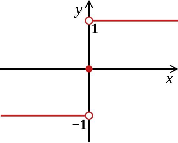
This is harsh (since an outcome of 0.49 and 0.51 lead to different values), and we cannot apply gradient descent on this function. For this reason, for binary classification, for example, we’ll tend to use a sigmoid activation function. Using a sigmoid activation will assign the value of a neuron to either 0 if the output is smaller than 0.5, or 1 if the neuron is larger than 0.5. The sigmoid function is defined by : \(f(x) = \frac {1} {1 + e^{-u}}\)

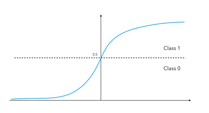
This activation function is smooth, differentiable (allows back-propagation) and continuous. We don’t have to output a 0 or a 1, but we can output probabilities to belong to a class instead. If you’re familiar with it, this version of the perceptron is a logistic regression with 0 hidden layers.

Some details

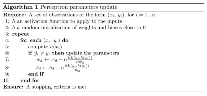
A given observation can be either well classified, or in the wrong class. As in most optimization problems, we want to minimize the cost, i.e the sum of the individual losses on each training observation. A pseudo-code corresponding to our problem is :

In the most basic framework of Minsky and Papert perceptron, we consider essentially a classification rule than can be represented as :

\[g(x) = sig({\alpha + \beta^tx})\]

where :

the bias term is \({\alpha}\)
the weights on each neuron is \({\beta}\)
the activation function is sigmoid, denoted as \(sig\).

We need to apply a stochastic gradient descent. The perceptron “learns” how to adapt the weights using backpropagation. The weights and bias are firstly set randomly, and we compute an error rate. Then, we proceed to backpropagation to adjust the parameters that we did not correctly identify, and we start all over again for a given number of epochs.

We will further detail the concepts of stochastic gradient descent and backpropagation in the context of Multilayer Perceptron.

Even the Minsky and Papert perceptron has a major drawback. If the categories are linearly separable for example, it identifies a single separating hyper-plane without taking into account the notion of margin we would like to maximize. This problem is solved by the Support Vector Machine (SVM) algorithm.

Logical operators

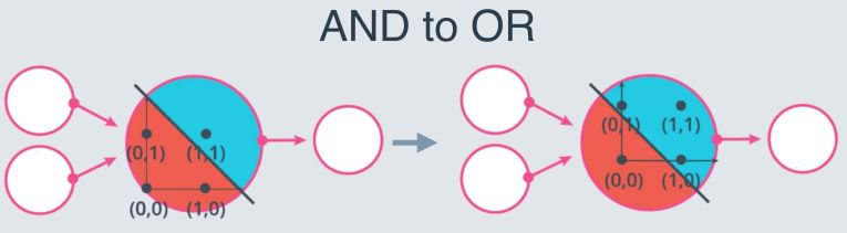
Perceptron can be used to represent logical operators. For example, one can represent the perceptron as an “AND” operator.

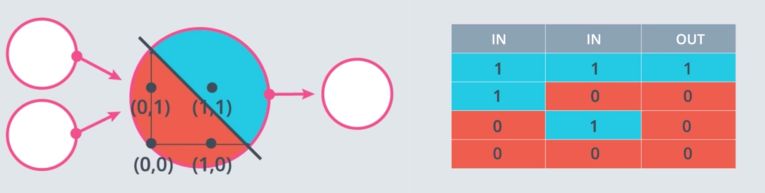
A simple “AND” perceptron can be built in the following way :

weight1 = 1.0
weight2 = 1
bias = -1.2

linear_combination = weight1 * input_0 + weight2 * input_1 + bias
output = int(linear_combination >= 0)

Where input_0 and input_1 represent the two feature inputs. We are shifting the bias by 1.2 to isolate the positive case where both inputs are 1.

However, solving the XOR problem is impossible :

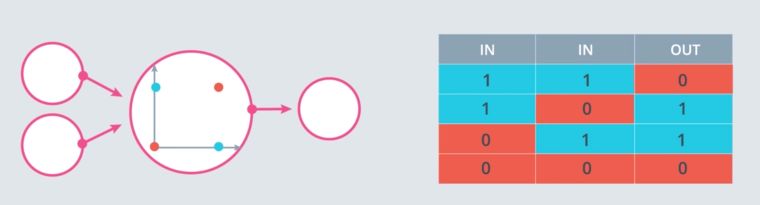
This is why Multi-layer perceptrons were introduced.

Implementation in Keras

In Keras, it is extremely easy to build a Perceptron :

from keras.models import Sequential
model = Sequential()
model.add(Dense(1, input_dim=6, activation='sigmoid'))

model.compile(loss='categorical_crossentropy', optimizer='adam', metrics=['accuracy'])
model.fit(X_train, y_train, epochs=20,batch_size=128)

Implementation in Tensorflow

Using the famous MNIST database as an example, a perceptron can be built the following way in Tensorflow. This simple application heads an accuracy of around 80 percents. This example is taken from the book: “Deep Learning for Computer Vision” by Dr. Stephen Moore, which I recommend. The following code is in Tensorflow 1 :

# Imports
from tensorflow.examples.tutorials.mnist import input_data
import tensorflow as tf
mnist_data = input_data.read_data_sets('MNIST_data', one_hot=True)

input_size = 784 # (28*28 flattened images)
no_classes = 10
batch_size = 100
total_batches = 200

x_input = tf.placeholder(tf.float32, shape=[None, input_size])
y_input = tf.placeholder(tf.float32, shape=[None, no_classes])
weights = tf.Variable(tf.random_normal([input_size, no_classes]))
bias = tf.Variable(tf.random_normal([no_classes]))

logits = tf.matmul(x_input, weights) + bias

softmax_cross_entropy = tf.nn.softmax_cross_entropy_with_logits(labels=y_input, logits=logits)
loss_operation = tf.reduce_mean(softmax_cross_entropy)
optimiser = tf.train.GradientDescentOptimizer(learning_rate=0.5).minimize(loss_operation)

Then create and run the training session :

session = tf.Session()
session.run(tf.global_variables_initializer())

for batch_no in range(total_batches):
    mnist_batch = mnist_data.train.next_batch(batch_size)
    _, loss_value = session.run([optimiser, loss_operation], feed_dict={
        x_input: mnist_batch[0],
        y_input: mnist_batch[1]
    })
    print(loss_value)

And compute the accuracy on the test images :

predictions = tf.argmax(logits, 1)
correct_predictions = tf.equal(predictions, tf.argmax(y_input, 1))
accuracy_operation = tf.reduce_mean(tf.cast(correct_predictions, tf.float32))

test_images, test_labels = mnist_data.test.images, mnist_data.test.labels
accuracy_value = session.run(accuracy_operation, feed_dict={
    x_input: test_images,
    y_input: test_labels
})

print('Accuracy : ', accuracy_value)
session.close()

This heads an accuracy of around 80% which can be largely improved by the next techniques we are going to cover.

Conclusion : Next step, we are going to explore the Multilayer Perceptron!

Sources :

Télécom Paris, IP Paris Lecture on Perceptron
https://towardsdatascience.com/mcculloch-pitts-model-5fdf65ac5dd1
https://towardsdatascience.com/rosenblatts-perceptron-the-very-first-neural-network-37a3ec09038a
https://towardsdatascience.com/perceptron-the-artificial-neuron-4d8c70d5cc8d

The Rosenblatt’s Perceptron

Maël Fabien