
Let’s continue our work on image alignment. We shall cover further details on image warping.
For what comes next, we’ll work a bit in Python. Import the following packages :
import cv2
import numpy as np
from matplotlib import pyplot as plt
So far, we saw how to :
- detect features (Harris corner detector, Laplacian of Gaussians for blobs, difference of Gaussians for fast approximation of the LOG)
- the properties of the ideal feature
- the properties of the feature descriptor
- matching of local features
- feature distance metrics
We’ll cover into further details image alignment.
I. Image Warping
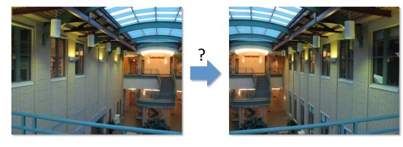
There is a geometric relationship between these 2 images :
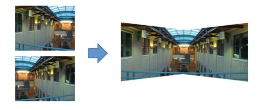
An image warping is a change of domain of an image : \(g(x) = f(h(x))\). This might include translation, rotation or aspect change. These changes are said to be global parametric warping: \(p' = T(p)\), since the transformation can easily be described by few parameters and is the same for every input point.
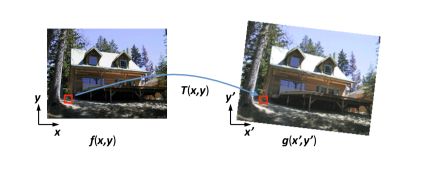
To build the transformed image, we usually apply an inverse-warping :
- for every pixel \(x'\) in \(g(x')\) :
- compute the source location \(x = \hat{h}(x')\)
- resample \(f(x)\) at location \(x\) and copy to \(g(x')\)
This allows \(\hat{h}(x')\) to be defined for all pixels in \(g(x')\).
1. Linear transformations
We’ll now cover the different types of linear transformations that we can apply to an image using inverse-warping.
a. Uniform Scaling
Scaling by factor \(s\) :
\[S = \begin{pmatrix} s & 0 \\ 0 & s \end{pmatrix}\]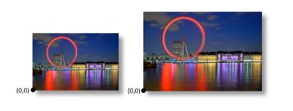
b. Rotation
Rotation by angle \(\theta\) :
\[R = \begin{pmatrix} cos \theta & - sin \theta \\ sin \theta & cos \theta \end{pmatrix}\]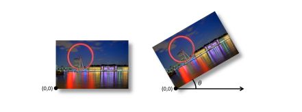
c. 2D Mirror about the Y-axis
\[T = \begin{pmatrix} -1 & 0 \\ 0 & 1 \end{pmatrix}\]d. 2D Miror accross line \(y = x\)
\[T = \begin{pmatrix} 0 & 1 \\ 1 & 0 \end{pmatrix}\]e. All 2D linear transformations
In summary, the linear transforms we can apply are :
- scale
- rotation
- shear
- mirror
The transformation should respect the following properties :
- origin maps origin
- lines map to lines
- parallel lines remain parallel
- ratios are preserved
- closed under composition
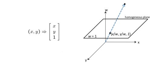
2. Translation
The trick is to add one more coordinate to build homogenous image coordinates.
3. Affine transformation
An affine transformation is any transformation that combines linear transformations and translations. For example :
\[\begin{pmatrix} x' \\ y' \\ w' \end{pmatrix} = \begin{pmatrix} a & b & c \\ d & e & f \\ 0 & 0 & 1 \end{pmatrix} \begin{pmatrix} x \\ y \\ w \end{pmatrix}\]In affine transformations, the origin does not always have to map the origin.
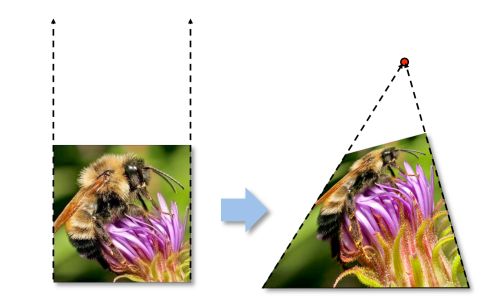
4. Homography
The Homography transform is also called projective transformation or planar perspective map.
\[H = \begin{pmatrix} a & b & c \\ d & e & f \\ g & h & 1 \end{pmatrix}\]Homographic transformations simply respect the following properties :
- lines map to lines
- closed under composition
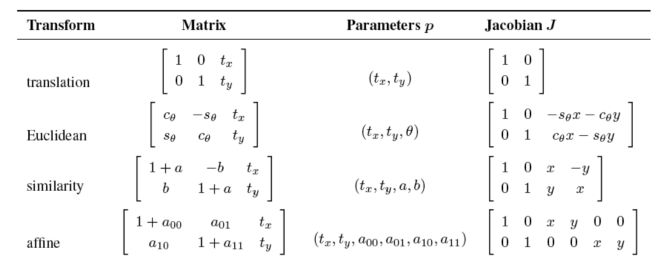
The different transformations can be summarized this way :
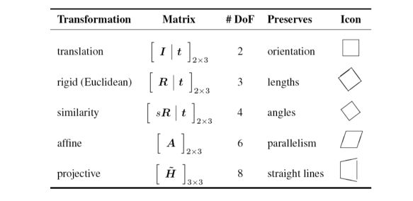
With homographies, points at infinity become finite vanishing points.
II. Computing transformations
Given a set of matches between images \(A\) and \(B\), we must find the transform \(T\) that best agrees with the matches.

1. Translation
The displacement of match \(i\) is \((x_i' - x_i, y_i' - y_i)\) where \(x_i' = x_i + x_t\) and \(y_i' = y_i + y_t\). We want therefore to solve :
\[(x_t, y_t) = ( \frac {1} {n} \sum_i x_i' - x_i, \frac {1} {n} \sum_i y_i' - y_i )\]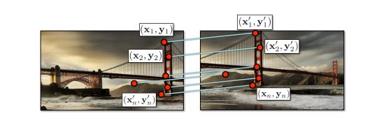
We face an overdetermined system of equations, which can be solved by least squares.
\[r_{x_i}(x_t) = x_i + x_t - x_i'\] \[r_{y_i}(y_t) = y_i + y_t - y_i'\]The goal is to minimize the sum of squared residuals :
\[C(x_t, y_t) = \sum_i (r_{x_i}(x_t)^2 + r_{y_i}(y_t)^2)\]We can rewrite the problem in matrix form :
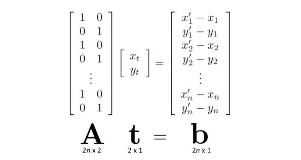
And the solution heads : \(t = (A^T A)^{-1} Ab\)
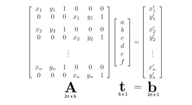
2. Affine transformation
\[\begin{pmatrix} x' \\ y' \\ w' \end{pmatrix} = \begin{pmatrix} a & b & c \\ d & e & f \\ 0 & 0 & 1 \end{pmatrix} \begin{pmatrix} x \\ y \\ w \end{pmatrix}\]We can write the residuals as :
\[r_{x_i}(a,b,c,d,e,f) = (ax_i + by_i + c) - x_i'\] \[r_{y_i}(a,b,c,d,e,f) = (dy_i + ey_i + f) - y_i'\]And rewrite the cost function as :
\[C(a,b,c,d,e,f) = \sum_i ( r_{x_i}(a,b,c,d,e,f)^2 + r_{y_i}(a,b,c,d,e,f)^2 )\]Which can be rewritten in matrix form as :
Let’s develop a more general formulation. We have \(x' = f(x,p)\) a parametric transformation. The Jacobian of the transformation \(f\) with respect to the motion parameters \(p\) determines the relationship between the amount of motion \(\Delta x = x' - x\) and the unknown parameters \(\Delta x = x' - x = J(x)p\) . We note that \(J = \frac {\delta f} {\delta p}\).
The sum of squared residuals is then :
\[E_{LLS} = \sum_i {\mid \mid J(x_i)p - \Delta x_i \mid \mid_2 }^2\]The solution yields :
\(Ap = b\) where :
- we define \(A = \sum_i J^T(x_i)J(x_i)\) the Hessian
- and \(b = \sum_i J^T(x_i) \Delta x_i\)
Up to now, we considered only a perfect matching accuracy. It’s however only rarely the case. We can weight the least squares problem :
\(E_{WLS} = \sum_i {\Sigma_i}^2 \mid \mid r_i \mid \mid\) . If the \(\delta_i\) are fixed, the solution to apply is : \(p = ( \sum^T A^T A \Sigma)^-1 \sigma^T Ab\) with \(\Sigma\) a matix containing for each observation the noise level.
**Conclusion **: I hope this article on image alignment, transformations, and warping was helpful. Don’t hesitate to drop a comment if you have any question.