
Have you ever wondered how panoramas are formed? How can several pictures be combined? This is done through local features.
For what comes next, we’ll work a bit in Python. Import the following packages :
import cv2
import numpy as np
from matplotlib import pyplot as plt
I. Local features
The key idea behind local features is to identify interest points, extract vector feature descriptor around each interest point and determine the correspondence between descriptors in two views.
Essentially, it can be illustrated this way :
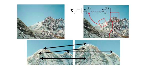
Global features describe the image as a whole to the generalize the entire object whereas the local features describe the image patches (key points in the image) of an object.
How can we find these local features? By following this simple procedure :
- detection: identify interest points
- tracking: search in a small neighborhood around each detected feature when images are taken from nearby points
- matching: determine the correspondence between descriptors in two views
We want our match to be reliable, invariant t geometric (translation, rotation, scale) and photometric (brightness, exposure) differences in the two views.
Local features are used for image alignment, panoramas, 3D reconstitution, motion tracking, object recognition, indexing, and database retrieval…
II. Detection
1. Detection theory
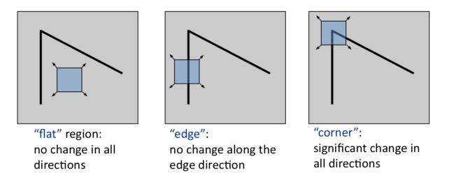
We want to look for unusual image regions. Textureless patches are nearly impossible to localize. We need to look for patches with large contrast changes, implying large gradients that vary along at least two orientations. This would be the case for corners for example.
Suppose we consider only a small window of pixels. We can define flat regions, edges, and corners the following way :
But how do we measure the change? What metric can we use?
We can sum up the squares differences (SSD) :
\[E(u,v) = \sum_{x,y ∈ W} [I(x+u, y+v) - I(x,y)]^2\]We can also compare two image patches using a weighted summed square difference :
\[E_{WSSD}(u) = \sum_{i} w(p_i) [I_1(p_i+u) - I_0(p_i)]^2\]where :
- the two images being compared are \(I_0\) and \(I_1\)
- the displacement vector is \(u(u_x, u_y)\)
- we have \(w(p)\) a spatially varying weighted function
We are interested in how stable this metric is with respect to small variations in \(u\). This is defined by the auto-correlation function :
\[E_{AC}(\Delta u) = \sum_{i} w(p_i) [I_1(p_i+ \Delta u) - I_0(p_i)]^2\]Using Taylor series : \(I_0 (p_i + \Delta u) ≈ I_0 (p_i) + ∇ I_0 (p_i) \Delta u\)
With a bit of calculus, we can appriximate the autocorrelation as :
\(E_{AC} (\Delta u) = \Delta u^T A \Delta u\) where \(A = \sum_u \sum_v w (u,v) \begin{pmatrix} {I_x}^2 & {I_x I_y} \\ {I_y I_x} & {I_y}^2 \end{pmatrix} = w \begin{pmatrix} {I_x}^2 & {I_x I_y} \\ {I_y I_x} & {I_y}^2 \end{pmatrix}\)
\(A\) can be interpreted as a tensor where the outer products of the gradients are convolved with a weighting function.
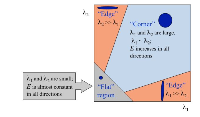
The eigenvalues of \(A\) carry information regarding uncertainty. Since \(A\) is symmetric, the eigenvalues of \(A\) reveal the amount of intensity change in the two principal orthogonal gradient directions in the window.
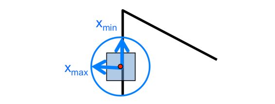
- direction of largest increase in E : \(x_{max}\)
- amount of increase in direction \(x_{max}\) : \(\lambda_{max}\)
- direction of smallest increase in E : \(x_{min}\)
- amount of increase in direction \(x_{min}\) : \(\lambda_{min}\)
How do we interpret the eigenvalues?
2. Harris’ corner detection
Let’s formalize the corner detection process using Harris’ method :
- compute the gradients at each point in the image
- compute \(A\) for each image window to get its corenerness scores
- compute the eigenvalues
- find points whose surrounding window gave a large corner response (f > threshold)
- take the points of local maxima and perform non-maximum suppression
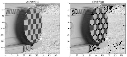
img = cv2.imread('vision_7.jpg', 0)
corn = img.copy()

dst = cv2.cornerHarris(img,3,5,0.22)

#result is dilated for marking the corners, not important
dst = cv2.dilate(dst,None)

# Threshold for an optimal value, it may vary depending on the image.
corn[dst>0.01*dst.max()]=0

plt.figure(figsize=(15,12))

plt.subplot(121)
plt.imshow(img,cmap = 'gray')
plt.title('Original Image')

plt.subplot(122)
plt.imshow(corn,cmap = 'gray')
plt.title('Corner Image')

plt.show()
The process of the Harris corner detection algorithm can be represented in the following way :
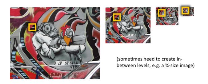
Harris Corner Detector is rotation invariant, but not scale-invariant (zooming out can make an edge become a corner for example).
How can we independently select interest points in each image such that the detections are repeatable across different scales? Well, we need to extract features at a variety of scales by using multiple resolutions in a pyramid and then matching features at the same level. We can also use a fixed window size with a Gaussian pyramid.
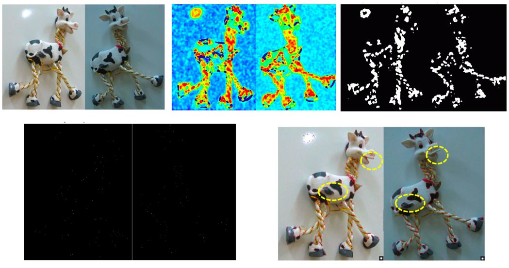
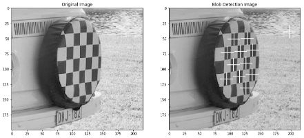
3. Blob detection
A Blob is a group of connected pixels in an image that shares some common property. Laplacian-of-Gaussian is a circularly symmetric operator for blob detection in 2D. We define the characteristic scale as the scale that produces the peak of Laplacian response.
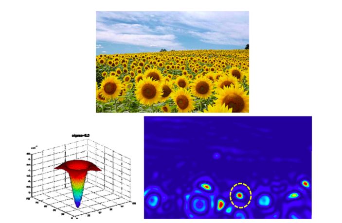
Interest points are local maxima in both position and scale.
detector = cv2.SimpleBlobDetector_create()
keypoints = detector.detect(img)

img2 = img.copy()
for marker in keypoints:
    img2 = cv2.drawMarker(img2, tuple(int(i) for i in marker.pt), color=(0, 255, 255))

plt.figure(figsize=(15,12))

plt.subplot(121)
plt.imshow(img,cmap = 'gray')
plt.title('Original Image')

plt.subplot(122)
plt.imshow(img2,cmap = 'gray')
plt.title('Blob Detection Image')

plt.show()
4. Ideal feature
The ideal feature should have the following properties :
- local, robust to occlusion and clutter
- invariant to certain transformation
- robust to noise, blur…
- distinctive so that individual features can be matched to a large database of objects
- quantify, so that many features can be generated for even small objects
- accurate, precise localization
- efficient, close to real-time
Other interest point detectors include :
- Hessian
- Lowe
- EBR, IBR
- MSER
- …
III. Description
The ideal feature descriptor to extract vector feature descriptor around each interest point should be :
- repeatable (invariant/robust)
- distinctive
- compact
- efficient
A first step is to normalize the pixels value. However, this is still very sensitive to shifts or rotations…
1. Scale Invariant Feature Transform (SIFT) descriptor
We compute the gradient at each pixel in a 16 × 16 window around the detected keypoint, using the appropriate level of the Gaussian pyramid at which the key point was detected. Down weight gradients by a Gaussian fall-off function (blue circle) to reduce the influence of gradients far from the center. In each 4 × 4 quadrants, compute a gradient orientation histogram using 8 orientation histogram bins.
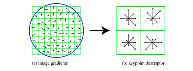
The resulting 128 non-negative values form a raw version of the SIFT descriptor vector.
It is also possible to apply a PCA at this level to reduce the 128 dimensions.
This is a great article of OpenCV’s documentation on these subjects.
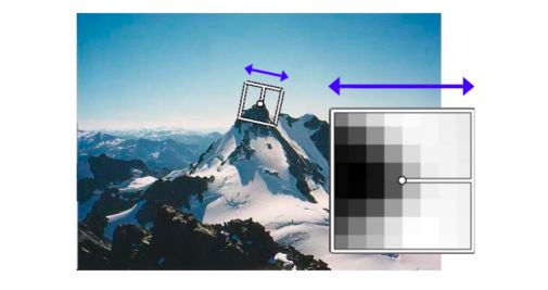
2. Multiscale Oriented Patches Descriptor (MOPS)
How can we make a descriptor invariant to the rotation?
We can rotate patch according to its dominant gradient orientation.
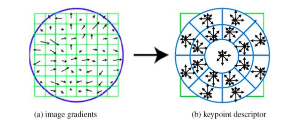
3. Other descriptors
- Gradient location-orientation histogram (GLOH) :
- Steerable filters
- moment invariants
- complex filters
- shape context
IV. Matching
We have detected interest points and extracted a vector feature descriptor around each point of interest. We now need to determine the correspondence between descriptors in two views.
To match local features, we need for example to minimize the SSD. The simplest approach would be to compare all key points and compare them all. We set a matching threshold value to identify the nearest neighbor to our point of interest.
How do we measure performance?
- True Positives
- False Negatives
- False Positives
- True Negatives
- Recall
- FPR
- Precision
- Accuracy
- ROC
- AUC
**Conclusion **: I hope this article on image features was helpful. Don’t hesitate to drop a comment if you have any question.