
How can you scale down an image? What other transformations can be applied?
For what comes next, we’ll work a bit in Python. Import the following packages :
import cv2
import numpy as np
from matplotlib import pyplot as plt
I. Image sub-sampling
The key idea in image sub-sampling is to throw away every other row and column to create a half-size image. When the sampling rate gets too low, we are not able to capture the details in the image anymore.
Instead, we should have a minimum signal/image rate, called the Nyquist rate.
Using Shannons Sampling Theorem, the minimum sampling should be such that :
\[f_s ≥ 2 f_{max}\]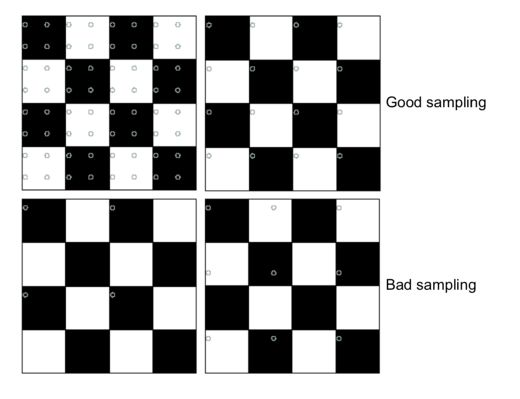
Image subsampling by dropping rows and columns will typically look like this :
The original image has frequencies that are too high. How can we solve this? Filter the image first, and then subsample.
To reduce the dimension, we apply a “decimation” :
\[g(i,j) = \sum_{i,j} f(k,l) h(i-k/r, j-l/r)\]II. Image up-sampling
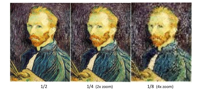
A classical method would be to repeat each row and column several times. This is called the Nearest Neighbor Interpolation. However, as you might expect, it’s not an efficient method.
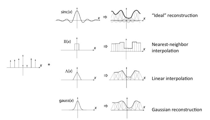
Recall that a digital image can be formed the following way :
\[F[x,y] = quantize (f(xd,yd))\]It’s a discrete point sampling of a continuous function. If we don’t know \(f\), we need to interpolate and guess an approximation. We convert \(F\) to a continuous function :
\(f_F(x) = F( \frac {x} {d})\) if \(\frac {x} {d}\) is an integer, 0 otherwise.
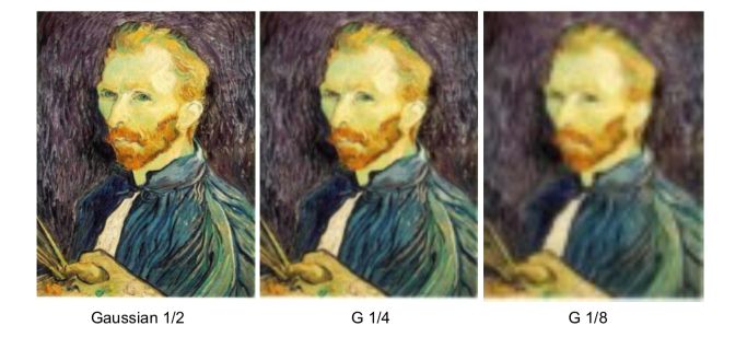
We then reconstruct the image by convolution with a reconstruction filter \(h\) : \(\hat{f} = h f_F\)
We can also use cubic filters which are quite common. To interpolate / upsample, we must select an interpolation kernel to convolve the image :
$ g(i,j) = \sum_{i,j} f(k,l) h(i-rk, j-rl) $$
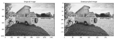
The up and down sampling can be achieved using the resize function in OpenCV :
res = cv2.resize(img, None, fx=0.2, fy=0.2, interpolation = cv2.INTER_CUBIC)

plt.figure(figsize=(15,12))

plt.subplot(121)
plt.imshow(img,cmap = 'gray')
plt.title('Original Image')

plt.subplot(122)
plt.imshow(res,cmap = 'gray')
plt.title('Downsampled Image')

plt.show()
The Laplacian Pyramid offers a multi-resolution representation.
- blur the image
- subsample the image
- subtract the low pass version of the original to get a band-pass Laplacian image
- the Laplacian pyramid has a perfect reconstitution.
This is pretty close to autoencoders in some sense.
III. Advanced filters
Other types of filters exist, and include :
- oriented filters for texture analysis, edge detection, compression… Apply many versions of the same filter to find the response.
- Another method: apply a few filters corresponding to angles, and interpolate. Steerable filters are a class of filters in which a filter of arbitrary orientation is synthesized as a linear combination of a set of basic filters.
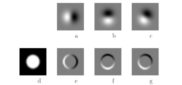
a. Steerable Filters
In Steerable filters, we’ll select a Gaussian filter and take the first derivative with respect to x and y. We combine the two derivatives (basis filters) into a linear combination (interpolation function).
This is an example of steerable filters :
b. Integral Images
The integral image is the running sum of all the pixels from the origin :
\[s(i,j) = \sum_k sum_l f(k,l) = s(i-1,j) + s(i,j-1) - s(i-1,j-1) + f(i,j)\]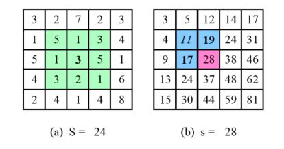
The information within an integral image can be represented in a so-called summed-area table.
c. Non-linear filters
We can, first of all, apply Median filtering to introduce non-linearity.
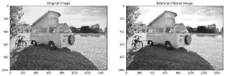
Bilateral Filtering
Bilateral filtering is a weighted filter kernel with a better outlier rejection. Instead of rejecting a fixed percentage, we reject (in a soft way) pixels whose values differ too much from the central pixel value.
blur = cv2.bilateralFilter(img,9,75,75)

plt.figure(figsize=(15,12))

plt.subplot(121)
plt.imshow(img,cmap = 'gray')
plt.title('Original Image')

plt.subplot(122)
plt.imshow(blur,cmap = 'gray')
plt.title('Bilateral Filtered Image')

plt.show()
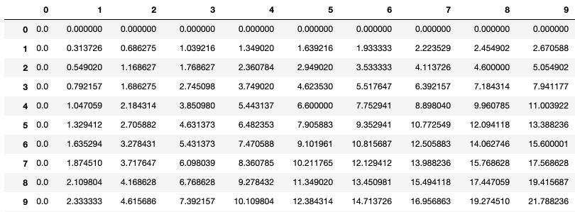
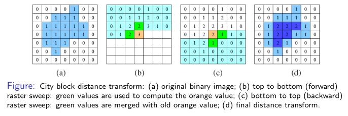
Distance Transform
In the distance transform, we compute the Manhattan Distance using :
- a Forward pass: each non-zero pixel is replaced by the minimum of 1 + the distance of its north or west neighbor
- a Backward pass: each non-zero pixel is replaced by the minimum of 1 + the distance of its south or east neighbor
Fourier analysis can be used to analyze the frequency characteristics of various filters. I won’t cover this part into much more details, but it’s an interesting topic and it links all filters (Gabor, Laplacian, Gaussian, box…).
Conclusion : I hope this article on image filtering was helpful. Don’t hesitate to drop a comment if you have any question.