
How is an image created? And what kind of filters can we apply to it? We’ll try to answer those questions in this article.
For what comes next, we’ll work a bit in Python. Import the following packages :
import cv2
import numpy as np
from matplotlib import pyplot as plt
I. How is an image created?
An image will always depend on :
- lighting conditions
- scene geometry
- surface properties
- camera optics
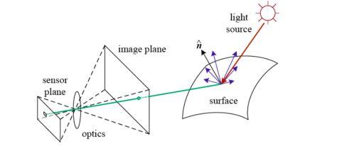
Using the imaging system, the photons that arrive at each cell are integrated and the digitized. An image appears as a grid of intensity values, corresponding to the value of each pixel.
0 = black, 255=white
An image can be compared to a function \(f : R^2 → R\) giving an intensity at each point \((x,y)\).
II. Image filtering
A filter can be seen as any kind of operator that can be applied to an image.
Filtering is often used for :
- image enhancement (denoise, resize…)
- extract information (texture, edges)
- detect patterns (template matching)
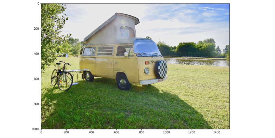
I’ll use a picture I have taken recently, but feel free to use any picture you’d like as long as there is some kind of color change or contrast in the image.
img = cv2.imread('vision_6.jpg')

b,g,r = cv2.split(img)
img = cv2.merge([r,g,b])

plt.figure(figsize=(12,8))
plt.imshow(img)
plt.show()
1. Noise reduction
A first way to reduce noise is to average out several noised images, but it typically requires a lot of images, which we generally do not have. We need to use smoothing filters to overcome this issue.
Smoothing filters have several properties :
- all values are positive
- they all sum to 1
- the amount of smoothing is proportional to the mask size
- it removes high-frequency components
a. Averaging
*Intuition *: Replace each pixel by the average of its neighbors. This assumes that neighboring pixels are similar and the noise is independent across pixels.
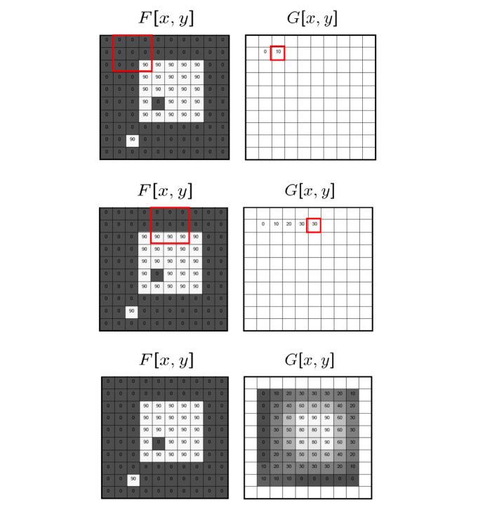
We define a filter size and apply a convolutional filter (moving average) on the input image.
Here’s a small animation of the filter evolution :
On an image, the process leads to the following averaged image :
The filter, when in size \(2 \times 2\) can be expressed as :
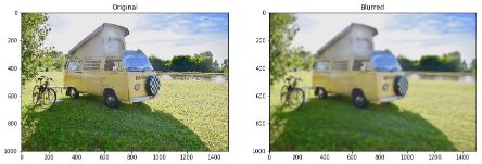
\[\frac {1} {4} \begin{pmatrix} 1 & 1 \\ 1 & 1 \end{pmatrix}\]This is already implemented in OpenCV. We’ll use a kernel size of \(15 \times 15\) :
blur = cv2.blur(img,(5,5))

plt.figure(figsize=(15,12))

plt.subplot(121)
plt.imshow(img)
plt.title('Original')

plt.subplot(122)
plt.imshow(blur)
plt.title('Blurred')

plt.show()
Another way to compute smoothing is to apply a Median Filtering, in which we take the median of all pixels within the kernel window. This is also really easy in OpenCV :
median = cv2.medianBlur(img,5)
b. Linear Filtering
*Intuition *: This involved a weighted combination of pixels in the small neighborhood of the pixel we want to estimate.
\[g(i,j) = \sum_{k,l} f(i+k, j+l) h (k,l)\]We call \(h(k,I)\) a kernel, or mask, and the problem can be rewritten using the correlation/convolution operator : \(G = H ⊗ F\) .
In Python :
ddepth = -1

# Define the kernel
kernel_size = 15
kernel = np.ones((kernel_size, kernel_size), dtype=np.float32)
kernel /= (kernel_size * kernel_size)

dst = cv2.filter2D(img, ddepth, kernel)

plt.figure(figsize=(15,12))

plt.subplot(121)
plt.imshow(img)
plt.title('Original')

plt.subplot(122)
plt.imshow(dst)
plt.title('Blurred')

plt.show()

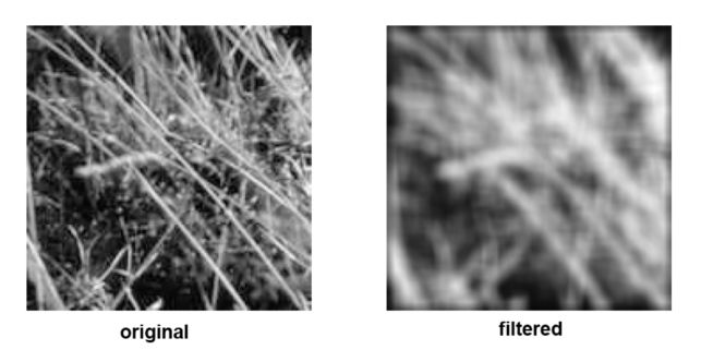
c. Gaussian Filtering
*Intuition *: We might want the pixels closer to the center to have more influence on the output. For this reason, we apply Gaussian filtering. It also removes high-frequency components from the image.
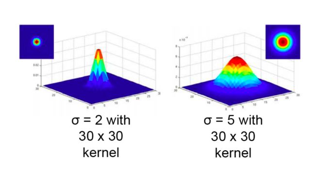
The Gaussian kernel is defined as :
\[h(u,v) = \frac {1} {2 \pi \sigma^2 } e^{ - \frac {u^2 + v^2} {\sigma^2}}\]The Gaussian Filtering is highly efficient at removing Gaussian noise in an image.
We can choose the size of the kernel or mask, and the variance, which determines the extent of smoothing.
In Python, Gaussian Filtering can be implemented using OpenCV :
blur = cv2.GaussianBlur(img,(15,15),10)

plt.figure(figsize=(15,12))

plt.subplot(121)
plt.imshow(img)
plt.title('Original')

plt.subplot(122)
plt.imshow(blur)
plt.title('Blurred')

plt.show()

2. Convolution filters
a. Convolution vs. Correlation
Convolution and Correlation are slightly different operations :
- Correlation :
- Convolution :
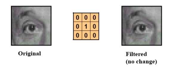
b. Examples of convolutions
a. Do nothing
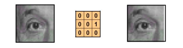
b. Shift the image
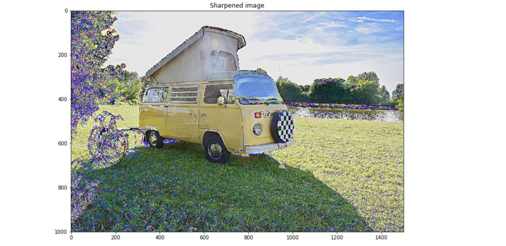
c. Sharpen an image
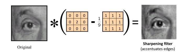
In Python, simply use :
plt.figure(figsize=(12,8))

plt.imshow(2*img - blur)
plt.title('Sharpened image')

plt.show()
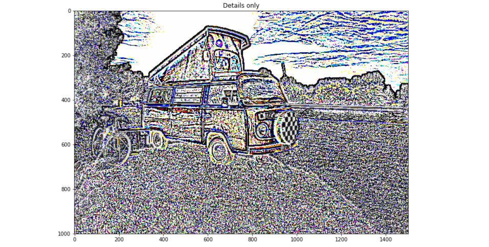
d. Find only the details of an image
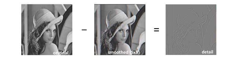
plt.figure(figsize=(12,8))

plt.imshow(img - blur)
plt.title('Edges only')

plt.show()
And apply this to our image :
The convolution is both commutative and associative. The Fourier transform of two convolved images is the product of their Fourier transforms. Both correlation and convolution are linear shift-invariant operators.
c. Separable convolution
A convolution requires \(K^2\) operations per pixel, where \(K\) is the size of the convolution kernel.
In many cases, this operation can be accelerated by first performing a 1D horizontal convolution followed by a 1D vertical convolution, requiring 2K operations. If this is possible, then the convolution kernel is called separable and is the outer product of 2 kernels: \(K = vh^T\).
A Kernel is separable if, in its Singular Value Decomposition (SVD), only one singular value is non-zero.
3. Edge Detection
a. What is an edge?
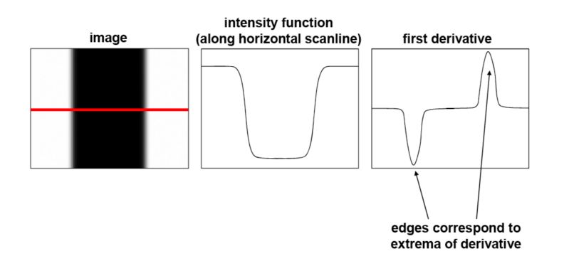
In edge detection, we map image from a 2d array to a set of curves or line segments. We look for strong gradients. An edge is a place of rapid change in the image intensity function.
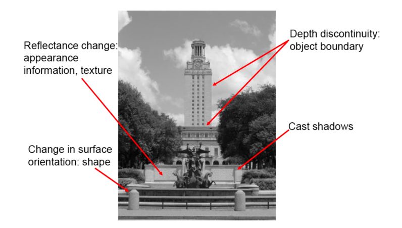
What causes an edge?
- reflectance change: appearance, information, texture
- change in surface orientation: shape
- shadows
- depth discontinuity: object boundary
b. Image gradient
How do we compute the derivative of a digital image \(F(x,y)\) with convolution ?
- Using the continuous image : \(\frac {\delta (x,y)} {\delta x} = {lim}_{ε→0} \frac {f(x+ε,y) - f(x)} {ε}\)
- Take discrete derivative \(\frac {\delta (x,y)} {\delta x} ≈ \frac {f[x+1,y] - f[x]} {1}\)
The gradient of an image is :
\[\Delta f = [ \frac {\delta f} {\delta x} \frac {\delta f} {\delta y} ]\]The gradient points in the direction of most rapid change in intensity. The partial derivative with respect to \(x\) is the horizontal direction, and the one with respect to \(y\) is the vertical direction.
The gradient direction is given by :
\[\theta = {tan}^{-1} ( \frac {\delta f} {\delta y} / \frac {\delta f} {\delta x})\]The edge strength is given by the magnitude :
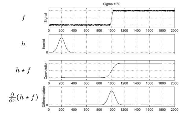
\[\mid \mid \Delta f \mid \mid = \sqrt { (\frac {\delta f} {\delta x})^2 (\frac {\delta f} {\delta y})^2 }\]Let’s consider a single row. We can plot the intensity as a function of position. This gives a signal.
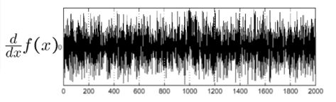
To identify the effect of noise, we smooth first and we look for picks in the differentiation of the smoothed original signal :
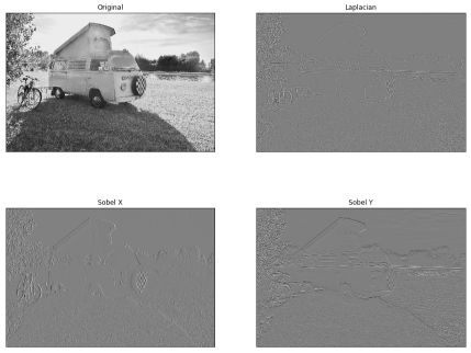
The filter we can apply in Python can be of various types :
- Sobel derivatives (X or Y), a joint Gaussian smoothing plus differentiation operation in which we can specify the direction (vertical, horizontal) of the derivatives.
- Band-pass filters such as Laplacian derivatives, obtained by convolving with a Gaussian filter and which filter low and high frequencies
laplacian = cv2.Laplacian(img,-3,ksize=9)
sobelx = cv2.Sobel(img,cv2.CV_64F,1,0,ksize=5)
sobely = cv2.Sobel(img,cv2.CV_64F,0,1,ksize=5)

plt.figure(figsize=(15,12))

plt.subplot(2,2,1),plt.imshow(img,cmap = 'gray')
plt.title('Original')

plt.subplot(2,2,2)
plt.imshow(laplacian,cmap = 'gray')
plt.title('Laplacian')

plt.subplot(2,2,3)
plt.imshow(sobelx,cmap = 'gray')
plt.title('Sobel X')

plt.subplot(2,2,4)
plt.imshow(sobely,cmap = 'gray')
plt.title('Sobel Y')

plt.show()
c. Find edges with Canny Edge Detector
A common way to find edges is to use the Canny Edge Detector :
- filter an image with a derivative of Gaussian
- find magnitude and orientation of the gradient
- non-maximum suppression: check if a pixel is a local maximum along gradient direction (requires interpolation)
- define 2 thresholds, low and high, and use the high to start edge curves and the low one to continue them
img = cv2.imread('vision_6.jpg', 0)

edges = cv2.Canny(img,300,300)
plt.figure(figsize=(15,12))

plt.subplot(121)
plt.imshow(img,cmap = 'gray')
plt.title('Original Image')

plt.subplot(122)
plt.imshow(edges,cmap = 'gray')
plt.title('Edge Image')

plt.show()
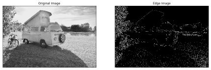
Canny edge detector does however not work that well on images such as this one, in which we have several trees and a lot of different textures.
Conclusion : I hope this article on image filtering was helpful. Don’t hesitate to drop a comment if you have any question.