Run ML models in SQL with BigQuery ML - Week 1 Module 3

In Google Cloud, one can build Machine Learning models straight into BigQuery, using SQL! Through this module, we will create Demand forecasting models using BigQuery ML.

Introduction to BigQuery

BigQuery is an easy to use Data Warehouse. It’s a petabyte-scale fully-managed service, and has several advantages :

• it’s serverless
• it offers flexible pricing models
• data encryption and security for regulatory requirements (restrictions on columns and row visibility
• geospatial data types and functions
• foundation for BI and AI

It’s a common workload to prototype ML models rapidly, and it is the bridge for data analysts and all users to your data.

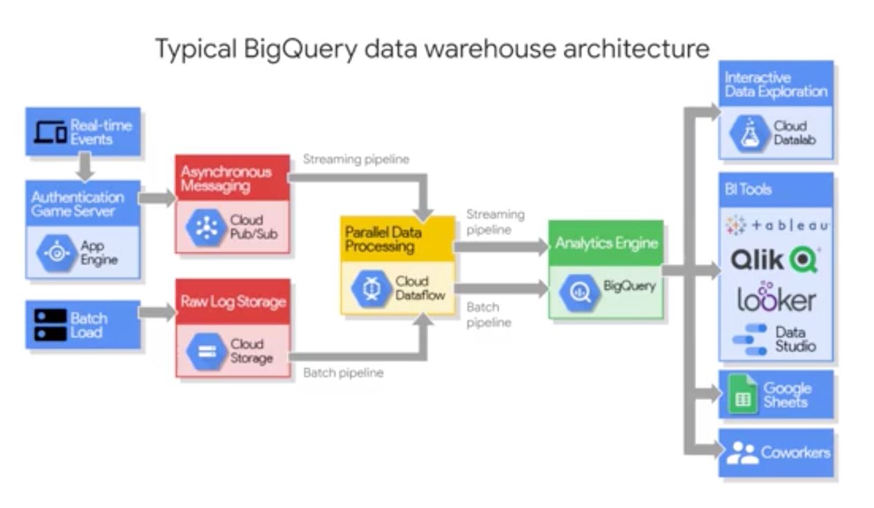
Big Query is essentially both a fast SQL query engine (BigQuery Query Service), and a managed storage for datasets (BigQuery Storage Service). Both services are fully managed and linked by a Petabit network.

The storage service relies on Google Colossus file storage system. This storage system also powers Google Photos for example. This storage service can do both :

• bulk data ingestions (huge amount of data)
• and streaming data ingestion (real-time data)

To launch a Query service, you can do it :

• through the command line
• through the WebUI
• through 7 REST APIs

The Query Service runs interactive or batch queries. It can connect to CSV files in Cloud Storage, but also to other services through connectors (Cloud Dataproc or Google Sheets for example).

Both services run together to optimize the syntax of the SQL query that is running.

BigQuery offers free monthly processing for up to 1TB.

BigQuery Query Service

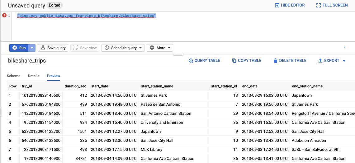
From the Query Editor, we’ll explore San Francisco bike-sharing data :

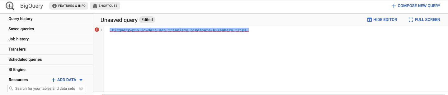
Type the following command (with the back-hyphens) :

 `bigquery-public-data.san_francisco_bikeshare.bikeshare_trips`

This is the link to the data. On macOS, simply hold the Command button, and click on the link of the data :

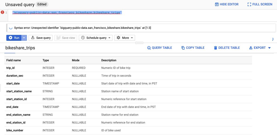
It opens a description of the table, gives you details about the number of rows, the size of the file… You can click on the Preview tab, without even running a query, to see the first 100 rows of the dataset.

If you click on the “Query table” button, it creates the default SQL format query :

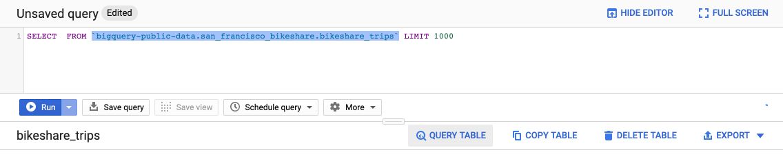
If you don’t want to type the name of the columns in the SELECT query, you can click on the column names from the Schema.

An example query would be :

SELECT trip_id, start_station_name FROM `bigquery-public-data.san_francisco_bikeshare.bikeshare_trips` LIMIT 1000

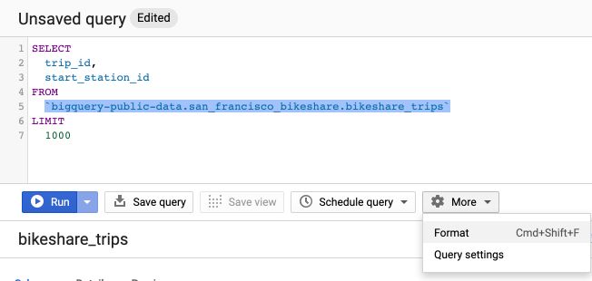
If you click on the Format button, it automatically re-formats the SQL query in a nice way :

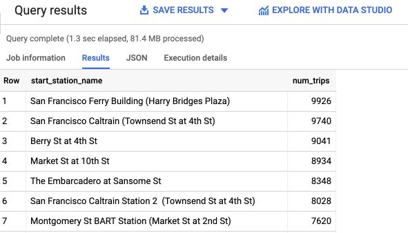
To get the stations in which we have the most rentals, we can run the following command :

# Top 10 station by Volume
SELECT
    start_station_name,
COUNT(trip_id) AS num_trips
FROM
    `bigquery-public-data.san_francisco_bikeshare.bikeshare_trips`
GROUP BY
    start_station_name
ORDER BY
    num_trips DESC
LIMIT
    1000

To filter only on rentals that occurred after 2017, apply a filter on the WHERE :

# Top 10 station by Volume since 2018
SELECT
    start_station_name,
COUNT(trip_id) AS num_trips
FROM
    `bigquery-public-data.san_francisco_bikeshare.bikeshare_trips`
WHERE
    start_date > '2017-12-31 00:00:00 UTC'
GROUP BY
    start_station_name
ORDER BY
    num_trips DESC
LIMIT
    1000

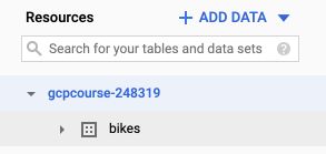
We can save a query as a Table to get a static table in the result (not a view). To do so, create an empty database in your project’s resources. I called mine bikes. Your architecture should be as follows :

To save a table, simply add a CREATE OR REPLACE argument at first :

# Top 10 station by Volume since 2018
CREATE OR REPLACE TABLE bikes.after_2017
SELECT
    start_station_name,
COUNT(trip_id) AS num_trips
FROM
    `bigquery-public-data.san_francisco_bikeshare.bikeshare_trips`
WHERE
    start_date > '2017-12-31 00:00:00 UTC'
GROUP BY
    start_station_name
ORDER BY
    num_trips DESC
LIMIT
    1000

The table is then added to the bikes database! To create a view, simply switch REPLACE table by VIEW :

# Top 10 station by Volume since 2018
CREATE OR REPLACE VIEW bikes.after_2017
SELECT
    start_station_name,
COUNT(trip_id) AS num_trips
FROM
    `bigquery-public-data.san_francisco_bikeshare.bikeshare_trips`
WHERE
    start_date > '2017-12-31 00:00:00 UTC'
GROUP BY
    start_station_name
ORDER BY
    num_trips DESC
LIMIT
    1000

To further explore the data, you can use DataStudio since it has a BigQuery connector.

Let’s talk a little bit about IAM Project roles and security. There are several levels of content access managed through roles :

• Viewer: Can start a job in the project
• Editor: Can create a dataset in the project
• Owner: Can list all datasets in the project, delete and create datasets

Dataset users should have the minimum permissions needed for their role. We use separated projects or datasets for different environments (DEV, QA, PRD…)

We also audit roles periodically.

BigQuery Storage Service

In addition to super-fast a super-fast query system, BigQuery can also ingest data from a large variety of sources :

• Cloud Storage
• Google Drive
• Cloud Bigtable
• CSV, JSON…

BigQuery is automatically replicated, backed-up, set up to auto-scaling… It’s a fully managed service. You can also directly query files that are outside the scope of BigQuery Managed Storage, although it’s not as optimized as for the files inside the scope. This is typically useful when ingesting external datasets from other services of a company.

BigQuery also allows for streaming records through API. The max input file size is 1MB, and the max output is 1000 files per second per project (If need more, consider Cloud Bigtable). It allows querying data without waiting for a full batch load.

Big Query natively supports arrays as data types :

It also supports STRUCTs, that satisfy the notions of Normalization of our tables.

Insights from geographic data

BigQuery natively supports Geographic Information System (GIS) function to get insights from geographic data. To deal with GIS data in your SQL queries, apply the following template :

SELECT
    ST_GeogPoint(longitude, latitude) AS point,
    name
FROM
    `bigquery-public-data.noaa_hurricanes.hurricanes`
WHERE
    name LIKE '%MARIA%'
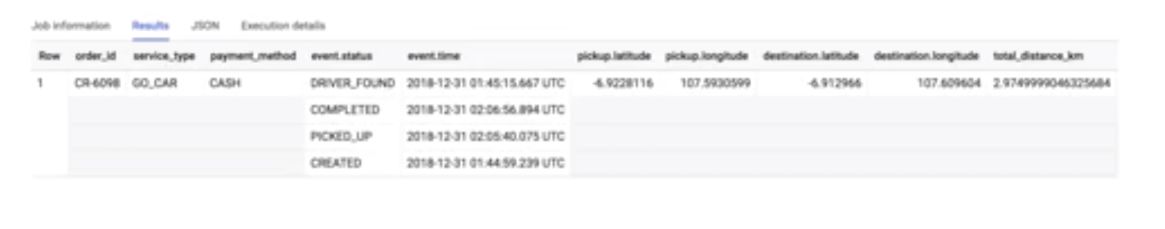
    AND ST_DWithin(st_geogfromtext('POLYGON((-179 26, -179 48, -10 48, -10 26, -100 -10.1, -179 26))'), ST_GeogPoint(longitude, latitude), 10)

This query creates a table of the geographic points of all hurricanes names MARIA within a given region, using the NOAA dataset.

To plot it, we can use GeoViz, a BigQuery tool that uses Google Map API. Access the tool here : https://bigquerygeoviz.appspot.com/.

Then, select your project ID and paste your SQL Query :

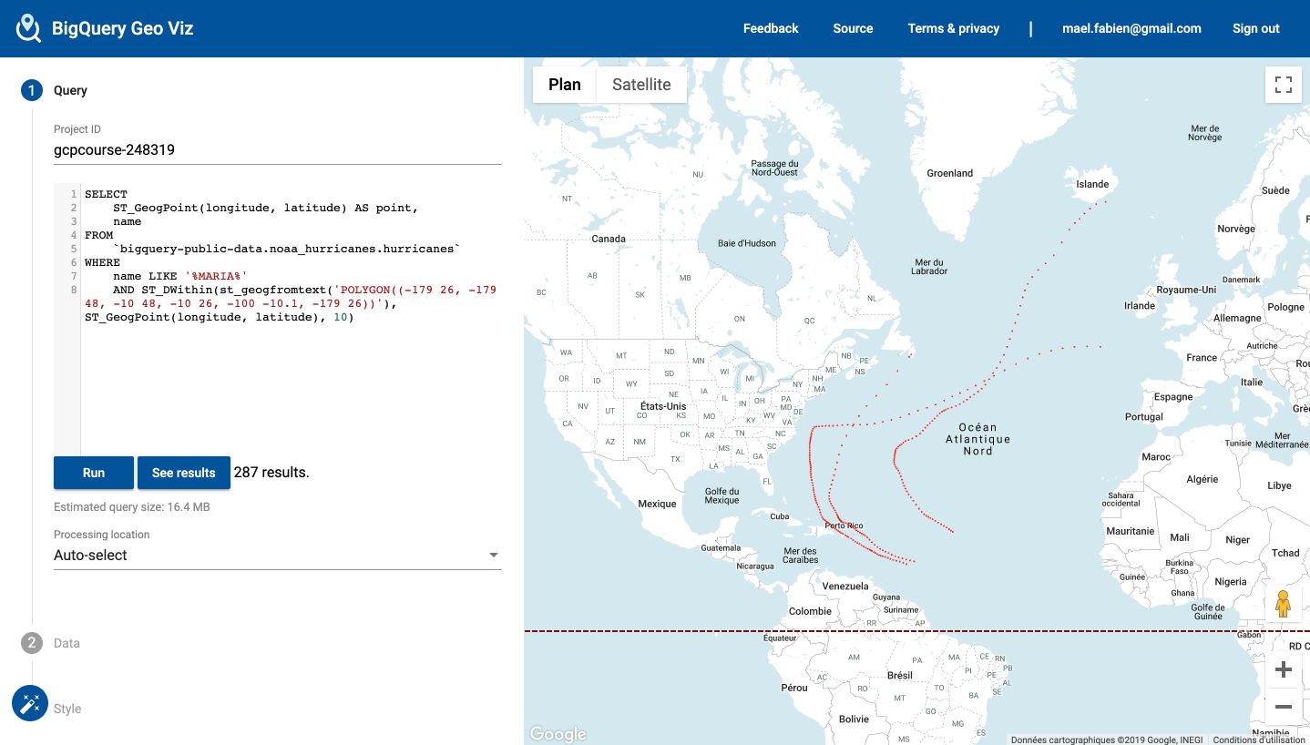
This is only a basic exploration in GeoViz, but the tool is really powerful.

BigQuery ML

More than 60% of ML models in Google operate on structured data. CNNs and LSTMs represent up to 35 % of the rest.

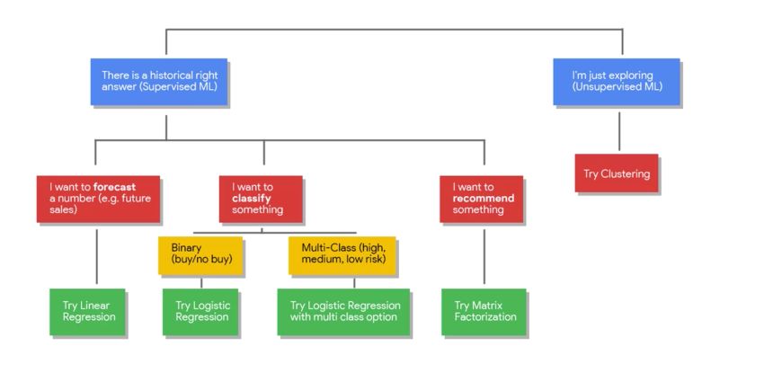
As a general guideline, here’s the most simple type of model you should consider in each case :

Here’s a scenario of lifetime value (how much profit we can expect from a customer) prediction on Google E-commerce datasets. The goal is to target high-value customers.

We have the following columns :

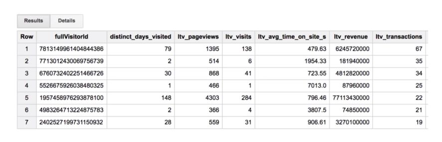
BigQuery ML will handle the train and test split. The 2 majors steps are to build the model and to fit it. The learning rate is auto-tuned. It also handles regularization.

The models currently supported in BigQuery ML are the following :

• Linear Regression
• Binary and Multiclass Logistic Regression

Other models are currently being added. Other interesting features are :

• Built-in model evaluation for standard metrics
• Model weight inspection
• Feature distribution analysis

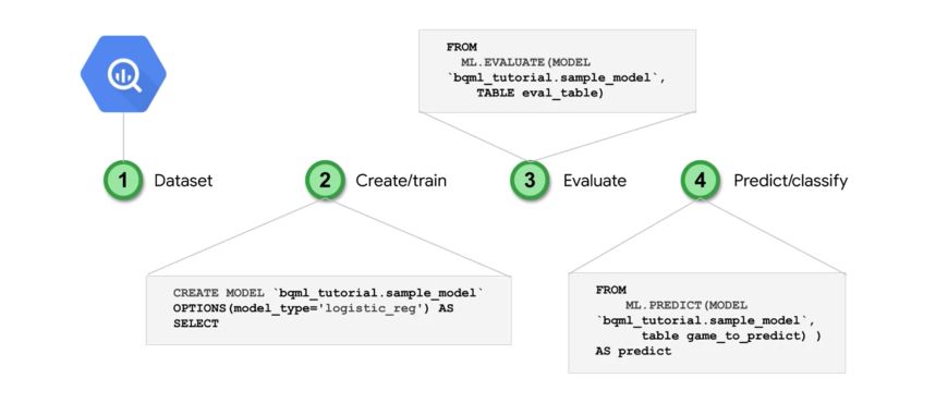
Here are the key steps in the model creation :

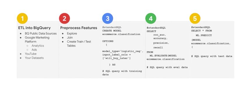
The key steps to build the model are essentially :

CREATE MODEL
ML.EVALUATE
ML.PREDICT

Key features

Model creation :

CREATE OR REPLACE MODEL
    `mydataset.mymodel`
OPTIONS
    ( model_type='linear_reg',
    input_label_cols='sales',
    ls_init_learn_rate=.15,
    l1_reg=1,
    max_iterations=5 ) AS

View features information :

SELECT
    *
FROM
    ML.FEATURE_INFO(MODEL
`bracketology.ncaa_model`)

Training progress :

SELECT
    *
FROM
    ML.TRAINING_INFO(MODEL
`bracketology.ncaa_model`)

Inspect the model weights :

SELECT
    category, 
    weight
FROM
    UNNEST((
        SELECT
            category_weights
        FROM
            ML.WEIGHTS(MODEL
        `bracketology.ncaa_model`)
        WHERE
            processed_input = 'seed'))
    features like 'school_ncaa'
        ORDER BY weight DESC

Evaluate a model :

SELECT
    *
FROM
    ML.EVALUATE(MODEL
`bracketology.ncaa_model`)

Make batch predictions :

CREATE OR REPLACE TABLES `bracketology.predictions`
AS (

SELECT * FROM ML.PREDICT(MODEL
`bracketology.ncaa_model`,

(SELECT * FROM `data-to-insights.ncaa.2018_tournament_results`)
)
)