Google now offers TPUs on Google Colaboratory. In this article, we’ll see what is a TPU, what TPU brings compared to CPU or GPU, and cover an example of how to train a model on TPU and how to make a prediction.

What is a TPU?

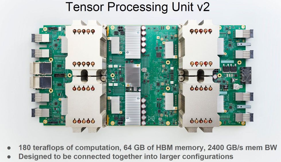
TPU stands for Tensor Processing Unit. It is an AI accelerator application-specific integrated circuit (ASIC). TPUs have been developed by Google in 2016 at Google I/O. However, TPUs have already been in Google data centers since 2015.

The chip is specifically designed for TensorFlow framework for neural network machine learning. Current TPU versions are already 3rd generation TPUs, launched in May 2018. Edge TPUs have also been launched in July 2018 for ML models for edge computing.

The TPUs have been designed, verified, built and deployed in just under 15 months, whereas typical ASIC development takes years.

If you’d like to know more on TPUs, check Google’s blog .

How do TPU work?

Quantization in neural networks

TPU use a technique called quantization to reduce execution time. Quantization is an optimization technique that uses an 8-bit integer to approximate an arbitrary value between a pre-set minimum and maximum value. Therefore, instead of using 16-bit or even 32-bit floating point operations, quantization dramatically reduces the computational requirements by maintaining quite similar precision of floating-point calculations.

The process of quantization is illustrated as follows on Google’s blog :

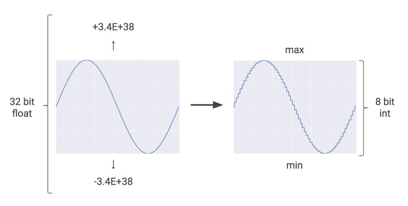
Memory usage drops when using quantization. For example, Google states that when applied to Inception image recognition challenge, memory usage gets compressed from 91MB to 23 MB.

TPUs use integer rather than floating-point operations, which highly reduces the hardware footprint and improves the computation time by up to 25 times.

TPU instruction set

TPU is designed to be flexible enough to accelerate computation times of many kinds of neural networks model.

Modern CPUs are influenced by the Reduced Instruction Set Computer (RISC) design style. The idea of RISC is to define simple instructions (load, store, add, multiply) and execute them as fast as possible.

TPUs use Complex Instruction Set Computer (CISC) style as an instruction set. CISC focus on implementing high-level instructions that run complex tasks such as multiply-and-add many times with each instruction.

What is a TPU made of?

TPUs are made of several computational resources :

Matric Multiplier Unit (MXU): 65,536 8-bit multiply-and-add units for matrix operations
Unified Buffer (UB): 24MB of SRAM that works as registers
Activation Unit (AU): Hardwired activation functions

Here’s an example of some high-levels instructions specifically designed for neural network inference that control how the MXU, UB, and AU work :

Read_Host_Memory : Read data from memory
Read_Weights : Read weights from memory
MatrixMultiply/Convolve: Multiply or convolve with the data and weights, accumulate the results
Activate : Apply activation functions
Write_Host_Memory : Write results to memory

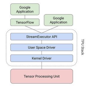
Google has created a compiler and software stack that translates API calls from TensorFlow graphs inti TPU instructions following this schema :

Parallel processing on MXU

Typical RISC processors provide instructions for multiplication or addition of numbers. They’re called scalar processors. It might, therefore, take time to execute large matrix operations.

Extensions of instructions set such as SSE and AVX allow matrix operations through vector processing where the same operation is conducted across a large number of data elements at the same time.

In TPU, Google designed the MXUas a matrix processor that processes hundreds of thousands of operations in a single clock cycle.

Systolic array

CPUs are made to run pretty much any calculation. Therefore, CPU store values in registers and a program sends a set of instructions to the Arithmetic Logic Unit to read a given register, perform an operation and register the output into the right register. This comes at some cost in terms of power and chip area.

For an MXU, matrix multiplication reuses both inputs many times, as illustrated below :

Data flows in through the chip in waves.

How efficient are TPUs?

The TPU MXU contains \(256 * 256 = 65'536\) ALUs. That means a TPU can process 65,536 multiply-and-adds for 8-bit integers every cycle. Because a TPU runs at 700MHz, a TPU can compute : \(65,536 × 700,000,000 = 46 × 10^{12}\) multiply-and-add operations or 92 Teraops per second in the matrix unit.

That being said, we can now move on to the practical part of this tutorial. Let’s use TPUs on Google Colab!

Connect the TPU and test it

First of all, connect to Google Colab : https://colab.research.google.com/ and create a new notebook in Python 3.

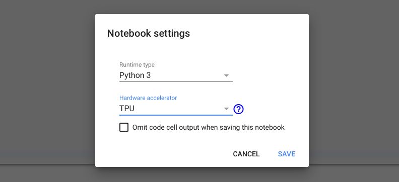
The first step is to modify the hardware of your notebook :

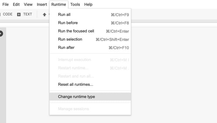
Switch the hardware accelerator to TPU :

Now, we’ll test if the TPU is well configured on the notebook :

import os
try:
    device_name = os.environ['COLAB_TPU_ADDR']
    TPU_ADDRESS = 'grpc://' + device_name
    print('Found TPU at: {}'.format(TPU_ADDRESS))
except KeyError:
    print('TPU not found')

If everything works well, you should observe something similar to :

Found TPU at: grpc://address

Load and process the data

We’ll import basic packages at first :

import numpy as np
import pandas as pd
import matplotlib.pyplot as plt

We’ll load the IMDB movie review dataset :

import tensorflow as tf
tf.set_random_seed(1)

from tensorflow.keras.datasets import imdb

Notice that we’ll always use the tensorflow.keras implementation, and not the keras implementation directly. Indeed, to run a model on TPU, it is essential.

We’ll have to process the data later on using tensorflow.keras :

from tensorflow.keras.models import Sequential
from tensorflow.keras.preprocessing import sequence
from tensorflow.keras.layers import Dense, Activation, Embedding, Dropout, Input, LSTM, Reshape, Lambda, RepeatVector
from tensorflow.keras import Model
from tensorflow.keras import backend as K
from tensorflow.keras.preprocessing.sequence import pad_sequences

In the IMDB movie review dataset, we’ll only consider the most common words :

top_words = 15000 
max_review_length = 250
INDEX_FROM = 3
epochs = 20
embedding_vector_length = 32

(X_train, y_train), (X_test, y_test) = imdb.load_data(num_words=top_words, index_from=INDEX_FROM)

X_train is now an array that contains lists of indexes. The indexes corresponding to the index of the word in the vocabulary. y_train contains labels (0 or 1) that describe the emotion of the review (positive or negative).

The reviews have different lengths. In order to normalize the length of the inputs, we “pad” the sequences to a defined length :

X_train = pad_sequences(X_train,max_review_length)
X_test = pad_sequences(X_test,max_review_length)

Build and fit the model

Alright, now the next step is to build a model that can predict whether a comment is negative or positive. LSTM’s can be useful since there is a dependency between the beginning and the end of a sentence. We’ll build a simple architecture accordingly with :

an Embedding layer
an LSTM layer
a Dense layer for the output

The model is really simple and does not prevent overfitting…

K.clear_session()
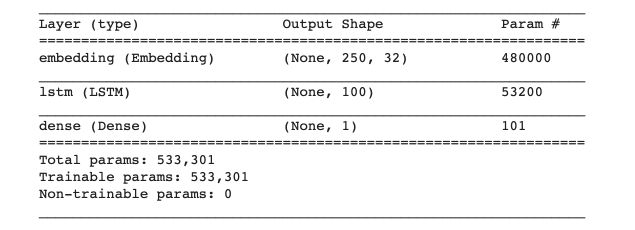
model = Sequential()

model.add(Embedding(top_words, embedding_vector_length, input_length=max_review_length))
model.add(LSTM(100))
model.add(Dense(1, activation='sigmoid'))

model.summary()

Then, compile the model :

model.compile(loss='binary_crossentropy', optimizer='adam', metrics=['accuracy'])

At that point, you may want to simply run model.fit. But you first need to transform your model in order to make it understandable by your TPU :

def model_to_tpu(model):
    return tf.contrib.tpu.keras_to_tpu_model( model, strategy=tf.contrib.tpu.TPUDistributionStrategy(tf.contrib.cluster_resolver.TPUClusterResolver(TPU_ADDRESS)))

Once this function is defined, just modify your model :

model = model_to_tpu(model)

Now, you can move on to the fitting of the model !

model.fit(X_train, y_train, epochs=epochs, batch_size=64, validation_data=(X_test, y_test))

Finally, we can save the model weights:

model.save_weights('./tpu_model.h5', overwrite=True)

We have already used our test set to evaluate the performance during the training. However, if you have a validation set for the validation accuracy during the training, you can evaluate the performance on your test set using :

model.evaluate(X_test, y_test, batch_size=128 * 8)

Notice that the batch_size is set to eight times of the model input batch_size since the input samples are evenly distributed to run on 8 TPU cores. This will require some modifications in prediction.

Performance of the model

In this section, I’ll try to compare the performance of Googe Colab TPU, GPU, and CPU on 20 epochs.

TPU performance

The TPU model has been fitted in less than 5 minutes. The average time per sample in each epoch is around 680 us.

Epoch 15/20
25000/25000 [==============================] - 17s 690us/sample - loss: 0.0344 - acc: 0.9888 - val_loss: 0.7723 - val_acc: 0.8302
Epoch 16/20
25000/25000 [==============================] - 17s 665us/sample - loss: 0.0196 - acc: 0.9946 - val_loss: 1.1661 - val_acc: 0.8204
Epoch 17/20
25000/25000 [==============================] - 18s 706us/sample - loss: 0.0105 - acc: 0.9972 - val_loss: 1.3740 - val_acc: 0.8103
Epoch 18/20
25000/25000 [==============================] - 17s 674us/sample - loss: 0.0102 - acc: 0.9972 - val_loss: 1.1836 - val_acc: 0.8290
Epoch 19/20
25000/25000 [==============================] - 17s 687us/sample - loss: 0.0352 - acc: 0.9889 - val_loss: 1.0536 - val_acc: 0.8258
Epoch 20/20
25000/25000 [==============================] - 17s 670us/sample - loss: 0.0293 - acc: 0.9915 - val_loss: 0.9991 - val_acc: 0.8302

The model has largely overfitted.

GPU performance

From the runtime menu, switch the hardware accelerator to GPU. The GPU is now way longer to run. A single epoch takes around 5 minutes. The average computing time per sample in each epoche is now 12 ms. The overall model ran in around 2.5 hours.

This means that on average, the model on TPU runs 17 times faster than on GPU! This is pretty close to the 25X faster announced.

Regarding the performance of the model, the GPU model reaches higher results around 84.5 %.

One would need more iterations to assess whether the difference is significant or not. We can guess that on LSTM computations like this one with a large number of variables, quantization’s impact can be observed on the final result.

CPU performance

Well, if a model runs on 2 hours on a GPU, you have to be patient to run it on the CPU. LSTM models would typically run over a whole night, so I decided to not run it for the moment.

Make a prediction

If you try to predict a TPU, you might encounter this issue :

AssertionError: batch_size must be divisible by the number of TPU cores in use (6 vs 8)

As discussed above, since the samples are evenly distributed to run on 8 TPU cores, your sample to predict needs to have a shape that is a multiple of 8. This might be problematic. To overcome this problem, we’ll convert the model back to CPU :

model = model.sync_to_cpu()
y_pred = model.predict(X_test)

We now have the prediction of our model, but the model’s training is now around 20 times faster!

Conclusion : I hope this introduction to Google Colab TPU’s was helpful. If you have any question, don’t hesitate to drop a comment!

TPU survival guide on Google Colaboratory

Maël Fabien