
Let’s dive deeper into the features a hit song should have. We are using the Spotify API for this analysis.
The data
Here we send requests to the Spotify API to retrieve specific information on songs. The features retrieved from the API are the following.
- duration_ms: The duration of the track in milliseconds.
- key: The estimated overall key of the track. Integers map to pitches using standard Pitch Class notation. E.g. 0 = C, 1 = C♯/D♭, 2 = D, and so on. If no key was detected, the value is -1.
- mode: Mode indicates the modality (major or minor) of a track, the type of scale from which its melodic content is derived. Major is represented by 1 and minor is 0.
- time_signature: An estimated overall time signature of a track. The time signature (meter) is a notational convention to specify how many beats are in each bar (or measure).
- acousticness: A confidence measure from 0.0 to 1.0 of whether the track is acoustic. 1.0 represents high confidence the track is acoustic. The distribution of values for this feature looks like this: Acousticness distribution
- danceability: Danceability describes how suitable a track is for dancing based on a combination of musical elements including tempo, rhythm stability, beat strength, and overall regularity. A value of 0.0 is least danceable and 1.0 is most danceable. The distribution of values for this feature looks like this: Danceability distribution
- energy: Energy is a measure from 0.0 to 1.0 and represents a perceptual measure of intensity and activity. Typically, energetic tracks feel fast, loud, and noisy. For example, death metal has high energy, while a Bach prelude scores low on the scale. Perceptual features contributing to this attribute include dynamic range, perceived loudness, timbre, onset rate, and general entropy. The distribution of values for this feature looks like this: Energy distribution
- instrumentalness : Predicts whether a track contains no vocals. “Ooh” and “aah” sounds are treated as instrumental in this context. Rap or spoken word tracks are clearly “vocal”. The closer the instrumentalness value is to 1.0, the greater the likelihood the track contains no vocal content. Values above 0.5 are intended to represent instrumental tracks, but confidence is higher as the value approaches 1.0. The distribution of values for this feature looks like this: Instrumentalness distribution
- liveness: Detects the presence of an audience in the recording. Higher liveness values represent an increased probability that the track was performed live. A value above 0.8 provides a strong likelihood that the track is live. The distribution of values for this feature looks like this: Liveness distribution
- loudness: The overall loudness of a track in decibels (dB). Loudness values are averaged across the entire track and are useful for comparing relative loudness of tracks. Loudness is the quality of a sound that is the primary psychological correlate of physical strength (amplitude). Values typical range between -60 and 0 dB. The distribution of values for this feature looks like this: Loudness distribution
- speechiness : Speechiness detects the presence of spoken words in a track. The more exclusively speech-like the recording (e.g. talk show, audiobook, poetry), the closer to 1.0 the attribute value. Values above 0.66 describe tracks that are probably made entirely of spoken words. Values between 0.33 and 0.66 describe tracks that may contain both music and speech, either in sections or layered, including such cases as rap music. Values below 0.33 most likely represent music and other non-speech-like tracks. The distribution of values for this feature looks like this: Speechiness distribution
- valence: A measure from 0.0 to 1.0 describing the musical positiveness conveyed by a track. Tracks with high valence sound more positive (e.g. happy, cheerful, euphoric), while tracks with low valence sound more negative (e.g. sad, depressed, angry). The distribution of values for this feature looks like this: Valence distribution tempo float The overall estimated tempo of a track in beats per minute (BPM). In musical terminology, the tempo is the speed or pace of a given piece and derives directly from the average beat duration. The distribution of values for this feature looks like this: Tempo distribution
- tempo: The overall estimated tempo of the section in beats per minute (BPM). In musical terminology, the tempo is the speed or pace of a given piece and derives directly from the average beat duration.
- key : The estimated overall key of the section. The values in this field ranging from 0 to 11 mapping to pitches using standard Pitch Class notation (E.g. 0 = C, 1 = C♯/D♭, 2 = D, and so on). If no key was detected, the value is -1.
- mode: integer Indicates the modality (major or minor) of a track, the type of scale from which its melodic content is derived. This field will contain a 0 for “minor”, a 1 for “major”, or a -1 for no result. Note that the major key (e.g. C major) could more likely be confused with the minor key at 3 semitones lower (e.g. A minor) as both keys carry the same pitches.
- mode_confidence: The confidence, from 0.0 to 1.0, of the reliability of the mode.
- time_signature : An estimated overall time signature of a track. The time signature (meter) is a notational convention to specify how many beats are in each bar (or measure). The time signature ranges from 3 to 7 indicating time signatures of “3/4”, to “7/4”.
import requests, json, logging
import pandas as pd
import base64
import six

def get_info(song_name = 'africa', artist_name = 'toto', req_type = 'track'):
    client_id = '***'
    client_secret = '***'
    auth_header = {'Authorization' : 'Basic %s' % base64.b64encode(six.text_type(client_id + ':' +                              client_secret).encode('ascii')).decode('ascii')}
    r = requests.post('https://accounts.spotify.com/api/token', headers = auth_header, data= {'grant_type': 'client_credentials'})
    token = 'Bearer {}'.format(r.json()['access_token'])
    headers = {'Authorization': token, "Accept": 'application/json', 'Content-Type': "application/json"}

    payload = {"q" : "artist:{} track:{}".format(artist_name, song_name), "type": req_type, "limit": "1"}

    res = requests.get('https://api.spotify.com/v1/search', params = payload, headers = headers)
    res = res.json()['tracks']['items'][0]
    year = res['album']['release_date'][:4]
    month = res['album']['release_date'][5:7]
    day = res['album']['release_date'][8:10]
    artist_id = res['artists'][0]['id']
    artist_name = res['artists'][0]['name'].lower()
    song_name = res['name'].lower()
    track_id = res['id']
    track_pop = res['popularity']

    res = requests.get('https://api.spotify.com/v1/audio-analysis/{}'.format(track_id), headers = headers)
    res = res.json()['track']
    duration = res['duration']
    end_fade = res['end_of_fade_in']
    key = res['key']
    key_con = res['key_confidence']
    mode = res['mode']
    mode_con = res['mode_confidence']
    start_fade = res['start_of_fade_out']
    temp = res['tempo']
    time_sig = res['time_signature']
    time_sig_con = res['time_signature_confidence']

    res = requests.get('https://api.spotify.com/v1/audio-features/{}'.format(track_id), headers = headers)
    res = res.json()
    acousticness =  res['acousticness']
    danceability = res['danceability']
    energy = res['energy']
    instrumentalness = res['instrumentalness']
    liveness = res['liveness']
    loudness = res['loudness']
    speechiness = res['speechiness']
    valence = res['valence']

    res = requests.get('https://api.spotify.com/v1/artists/{}'.format(artist_id), headers = headers)
    artist_hot = res.json()['popularity']/100

    return pd.Series([artist_name, song_name, duration, key,mode,temp,artist_hot,end_fade, start_fade, mode_con,key_con,time_sig,time_sig_con,acousticness,danceability,energy ,instrumentalness,liveness,loudness,speechiness,valence, year, month, day, track_pop], index = ['artist_name', 'song_name', 'duration','key','mode','tempo','artist_hotttnesss','end_of_fade_in','start_of_fade_out','mode_confidence','key_confidence','time_signature','time_signature_confidence','acousticness','danceability','energy' ,'instrumentalness','liveness','loudness','speechiness','valence','year','month', 'day', 'track_popularity'])
This function tests if a song request through the API is successful.
def test(song_name = 'africa', artist_name = 'toto', req_type = 'track'):
    client_id = '***'
    client_secret = '***'
    auth_header = {'Authorization' : 'Basic %s' % base64.b64encode(six.text_type(client_id + ':' + client_secret).encode('ascii')).decode('ascii')}
    r = requests.post('https://accounts.spotify.com/api/token', headers = auth_header, data= {'grant_type': 'client_credentials'})
    token = 'Bearer {}'.format(r.json()['access_token'])
    headers = {'Authorization': token, "Accept": 'application/json', 'Content-Type': "application/json"}

    payload = {"q" : "artist:{} track:{}".format(artist_name, song_name), "type": req_type, "limit": "1"}

    res = requests.get('https://api.spotify.com/v1/search', params = payload, headers = headers)
    if not res.json()['tracks']['items']:
        return False
    else:
        return True
This part of the code iterates over our dataset of hit songs (.csv file) to request the Spotify API and retrieve the audio features. Everything is gathered in a single data frame, and we create a feature by combining the mode confidence and the mode. We then proceeded to some data cleaning :
song_list = pd.read_csv('/Users/raphaellederman/Downloads/Tracks_Hackathon_treated (4).csv', sep = ';')
print(type(song_list['Track Name']))

rows= []
features = ['artist_name', 'song_name', 'duration','key','mode','tempo','artist_hotttnesss','end_of_fade_in','start_of_fade_out','mode_confidence','key_confidence','time_signature','time_signature_confidence','acousticness','danceability','energy' ,'instrumentalness','liveness','loudness','speechiness','valence','year','month', 'day', 'track_popularity']

for index, row in song_list.iterrows():
    print(row['Track Name'].replace('\'','') + ' - ' + row['Artist'])
    if test(row['Track Name'].replace('\'',''), row['Artist'], req_type = 'track') == True :
        rows.append(get_info(row['Track Name'].replace('\'',''), row['Artist'], req_type = 'track'))

data = pd.DataFrame(rows, columns=features)
data['mode_confidence'] = np.where(data['mode'] == 1, data['mode']* data['mode_confidence'], (data['mode']- 1)* data['mode_confidence'])
data = data.drop('mode', axis=1)

data_songs = data_songs.reset_index().drop(['index', 'artist_name', 'song_name'], axis=1).replace('', np.nan).dropna()
Exploratory data analysis
One of the best way to understand how features are related in a music is to build the correlation matrix :
import seaborn as sn
fig = plt.figure(figsize=(20, 20))
sn.heatmap(data.corr(),  annot=True)
plt.title('Correlation of every features', fontsize=20)
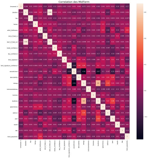
We are trying to predict how likely the artist is to be considered as a hot artist in 2019. Therefore, we focus on the variables that have a correlation of more than 0.1 or less than -0.1 with the artist Hotness.
features = [ 'duration', 'tempo', 'danceability', 'end_of_fade_in', 'start_of_fade_out','energy', 'speechiness','valence','track_popularity']
i=1
for feature in features :
plt.figure(figsize=(15,15))
plt.subplot(3,3, i )
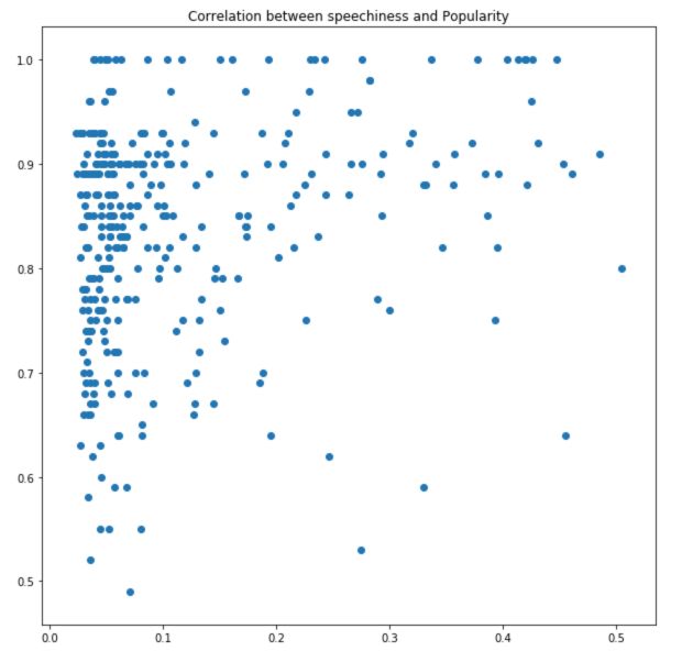
plt.scatter(data['artist_hotttnesss'], data[feature])
plt.title("correlation between artist_hotttnesss and " + feature)
i+=1
I won’t display all the graphs here, but one of the interesting relations is between artist hotness and the speechiness. This relation pretty much illustrates the popularity of rap artists. Indeed, rap tends to be a quite speechy music style.
The basic features
We tend to believe that taking the most popular features of each hit song of 2018 should be a pretty good start to make your next song a hit. If we focus on some features :
data.describe()
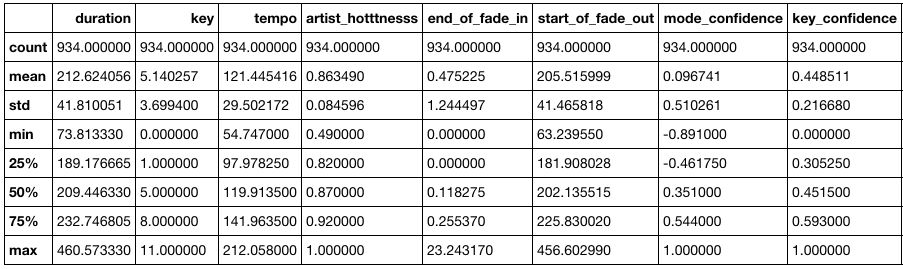
Among the most important features, we observe that the idea tempo should be around 120 BPM, and the ideal duration should be around 213 seconds.
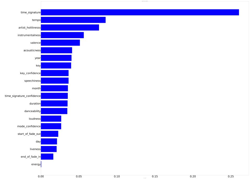
Feature importance
We used a Random Forest Regressor to evaluate feature importance when predicting the track popularity :
features_columns = [col for col in data.drop("track_popularity", axis = 1).columns]
X = data[features_columns].apply(pd.to_numeric, errors='coerce')
y = data['track_popularity'].apply(pd.to_numeric, errors='coerce')

# Split the data in order to compute the accuracy score
X_train, X_test, y_train, y_test = train_test_split(X, y, test_size=0.2, random_state=1)
We can construct a plot showing the importance of the features:
rnd_clf = RandomForestRegressor(n_estimators=100, n_jobs=-1, random_state=42)
rnd_clf.fit(X_train, y_train)

importances_rf = rnd_clf.feature_importances_
indices_rf = np.argsort(importances_rf)

n = len(indices_rf)
sorted_features_rf = [0] * n;
for i in range(0,n):
sorted_features_rf[indices_rf[i]] = features_columns[i]

plt.figure(figsize=(140,120) )
plt.title('Random Forest Features Importance')
plt.barh(range(len(indices_rf)), importances_rf[indices_rf], color='b', align='center')
plt.yticks(range(len(indices_rf)), sorted_features_rf)
plt.xlabel('Relative Importance')
plt.tick_params(axis='both', which='major', labelsize=100)
plt.tick_params(axis='both', which='minor', labelsize=100)

plt.show()
At that point, we were pretty much running short on time. We tried several regressors to predict of song popularity. The one that happened to work best was the XGBoost, but the overall training set was too small (which headed a 26% r-squared only…).
clf = xgboost.XGBRegressor(colsample_bytree = 0.44, n_estimators=30000, learning_rate=0.07,max_depth=9,alpha = 5)
model = clf.fit(X_train.drop(worst_features, axis=1), y_train)
pred = model.predict(X_test.drop(worst_features, axis=1))
score_rf = metrics.r2_score(y_test, pred)
print(score_rf)
Release time
At that point, we had all the ingredients of the perfect song, but when should the song be released? Spotify’s API gave us access to the release date of the hits in its charts.
s = pd.Series(data['month']).dropna()
fig, ax = plt.subplots(figsize = (12,12))
ax.hist(s, alpha=0.8, color='blue', bins = 25)
ax.xaxis.set_ticks(range(13))
ax.xaxis.set_ticklabels( [' ','Janvier', 'Fevrier', 'Mars', 'Avril', 'Mai', 'Juin', 'Juillet', 'Aout', 'Septembre', 'Octobre', 'Novembre', 'Decembre'])
plt.title("Historgram of the number of hit by month")
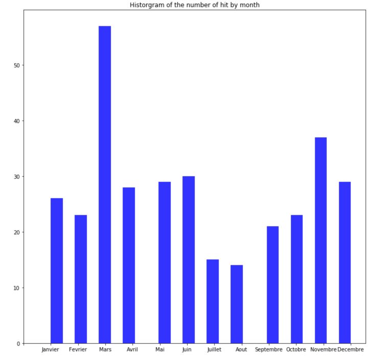
March looks great to launch your next hit ;)
**Conclusion **: Alright, this is all we had time to cover in this 10 hours Hackathon. Of course, we wanted to explore many more axis. At some point, we had to start focusing on the report to hand it and start preparing our pitch. I hope you enjoyed this series of articles!