
Earlier this year, at Telecom ParisTech, we had the opportunity to participate in a 10 hours Hackathon. The subject was pretty open: What will be the hit song of 2019?
We were working in groups of 5 and had 10 hours to hand in a Jupyter Notebook. I wanted to share this experience, and especially the way we organized the group project, and the outcomes.
The first 30 minutes
The first 30 minutes are the most important of the whole day. The questions you should answer in those first 30 minutes are the following :
- which data sets are you going to use?
- who will be responsible for what?
- are your data sources sufficient? Should you diversify?
- how will you break down the project?
This hackathon was centered on the storytelling we could build around our results, the prediction accuracy being only secondary. Therefore, we decided to break down the project in key questions, find a dataset that would support each or several questions. We planned to answer the following questions :
- Which country should you focus on?
- Who should you sing with?
- What should your nationality be?
- What kind of music should you play?
- What kind of lyrics should you write?
- How many words should you pronounce in a single song?
- Should you repeat words?
- What are the main words you should use?
- Should you write a positive or a negative song?
- What kind of mood should you express?
- What are the most important musical features of a top hit?
- Are we able to build a prediction from the features we extracted?
- Making a video clip on YouTube, worth it?
- When should the song be released?
A few imports before we start… (not all of them are useful at this step).
import pandas as pd
import numpy as np
import matplotlib.pyplot as plt
import os
import plotly.plotly as py
import plotly.graph_objs as go
import IPython.display as ipd
import requests
import lyricsgenius as genius
from glob import glob
import os.path as op
from nltk.corpus import stopwords
import re
import itertools
from wordcloud import WordCloud, STOPWORDS
from sklearn import model_selection
from sklearn.svm import LinearSVC
import pickle
from bs4 import BeautifulSoup
import seaborn as sns
from matplotlib import rc
from sklearn import linear_model
from sklearn.pipeline import Pipeline
from sklearn.preprocessing import PolynomialFeatures
import numpy as np
from sklearn.model_selection import train_test_split
from sklearn.ensemble import RandomForestRegressor
from sklearn.linear_model import LinearRegression
from sklearn.linear_model import LassoCV
from sklearn.ensemble import GradientBoostingRegressor
from sklearn import metrics
import requests, json, logging
import pandas as pd
import base64
import six
from sklearn import  linear_model
Which country should you focus on?
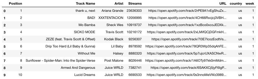
We tried to answer this question by looking at the total number of streams in the 10 regions of the world that listen to the most music. We downloaded data of streams from the Spotify Top 200 charts: https://spotifycharts.com/regional
Load datas from the Spotify Top Charts : https://spotifycharts.com/regional
folder = "**********/Hackathon/Total/"
onlyfiles = [f for f in os.listdir(folder) if os.path.isfile(os.path.join(folder, f))]
print("Working with {0} csv files".format(len(onlyfiles)))
We then gathered all files in a single data frame :
data = []

for file in onlyfiles :
    if file != '.DS_Store' :
        df = pd.read_csv(folder + file, skiprows=1)
        df['country'] = file[9:11]
        df['week'] = file[19:20]
        data.append(df)

data = pd.concat(data, axis=0)
We now need to group some rows, as you may have understood that the data are ordered per region per week.
data_country = data.groupby(['country'])[["Streams"]].sum().sort_values('Streams', ascending=True)
data_artists = data.groupby(['Artist'])[["Streams"]].sum().sort_values('Streams', ascending=False)
I like using Plotly for this kind of tasks, it allows a pretty visual representation of the data.
trace0 = go.Bar(
    x=data_country.index,
    y=data_country['Streams'],
    text=data_country['Streams'],
    marker=dict(
        color='rgb(158,202,225)',
        line=dict(
            color='rgb(8,48,107)',
            width=1.5,
        )
    ),
    opacity=0.6
)

data = [trace0]
layout = go.Layout(
    title='Regions of the world that consume most music',
)

fig1 = go.Figure(data=data, layout=layout)
py.iplot(fig1, filename='text-hover-bar')
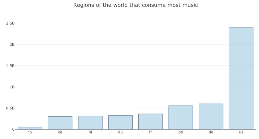
It looks pretty clear from this graph that the US market is by far the most important in terms of monthly music streams. Over the past month, the US market has consumed as much music streaming as Germany, Great Britain, France, Australia, Netherlands, Canada, and Japan together.
We were pretty short on time, but it could be interesting to take a look at the streams per person in all those regions.
Who should you sing with?
Plotting the same thing, but for the data_artists table heads :
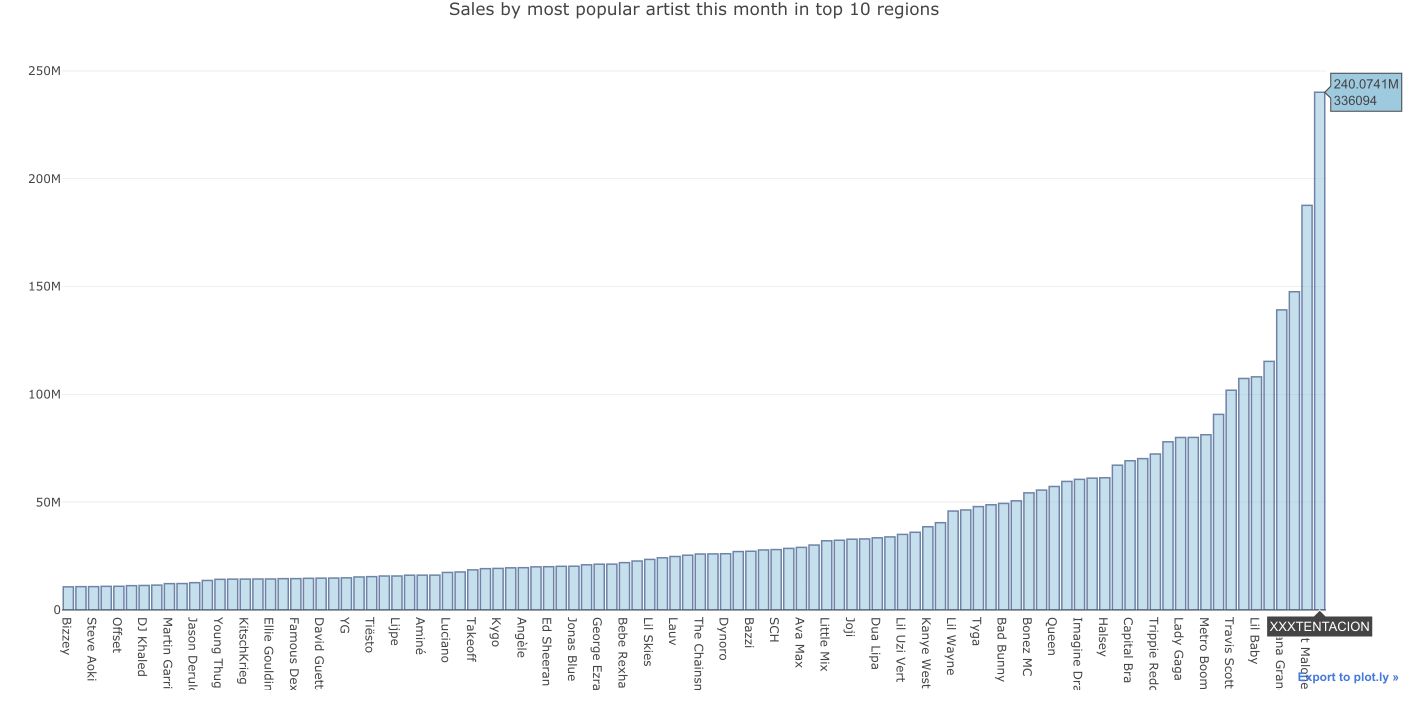
The top trending artist at the time this article is written is XXXTentacion. However, the young rapper passed away this summer, and his latest hits were revealed.
Otherwise, the next trending artists are :
- XXX Tentacion
- Post Malone
- Khalid
- Ariana Grande
- Juice WRLD
- Lil Baby
- Drake
- …
What should your nationality be?
We can expect that in some countries, the probability to become a top trending artist is higher than in others. Once again, we could have controlled for the population of each country to get a probability instead of the raw value.
Based on this list: https://www.thefamouspeople.com/singers.php, we have scrapped the most relevant data regarding the nationality of the most famous artists.
def _handle_request_result_and_build_soup(request_result):
    if request_result.status_code == 200:
    html_doc =  request_result.text
    soup = BeautifulSoup(html_doc,"html.parser")

    return soup

def _convert_string_to_int(string):
    if "K" in string:
        string = string.strip()[:-1]
        return float(string.replace(',','.'))*1000
    else:
        return int(string.strip())

def get_all_links_for_query(query):
    url = website + "/rechercher/"
    res = requests.post(url, data = {'q': query })
    soup = _handle_request_result_and_build_soup(res)
    specific_class = "c-article-flux__title"
    all_links = map(lambda x : x.attrs['href'] , soup.find_all("a", class_= specific_class))

    return all_links

def get_share_count_for_page(page_url):
    res = requests.get(page_url)
    soup = _handle_request_result_and_build_soup(res)
    specific_class = "c-sharebox__stats-number"
    share_count_text = soup.find("span", class_= specific_class).text

    return  _convert_string_to_int(share_count_text)


def get_popularity_for_people(query):
    url_people = get_all_links_for_query(query)
    results_people = []

    for url in url_people:
        results_people.append(get_share_count_for_page(website_prefix + url))

    return sum(results_people)

def get_name_nationality(page_url):
    res = requests.get(page_url)
    soup = _handle_request_result_and_build_soup(res)
    specific_class = "btn btn-primary btn-sm btn-block btn-block-margin"
    share_count_text = soup.find("a", class_= specific_class).text

    return  share_count_text
artists_dict = {}

for i in range(1, 17):
    website = 'https://www.thefamouspeople.com/singers.php?page='+str(i)

    res = requests.get(website)
    specific_class = "btn btn-primary btn-sm btn-block btn-block-margin"
    soup = _handle_request_result_and_build_soup(res)
    classes = soup.find_all("a", class_= specific_class)

    for i in classes:
        mini_array = i.text[:-1].split('(')
            artists_dict[mini_array[0]]=mini_array[1]

artists_df = pd.DataFrame.from_dict(artists_dict, orient='index', columns=['Country'])
artists_df.head(n=10)
Plotting the results, we get :
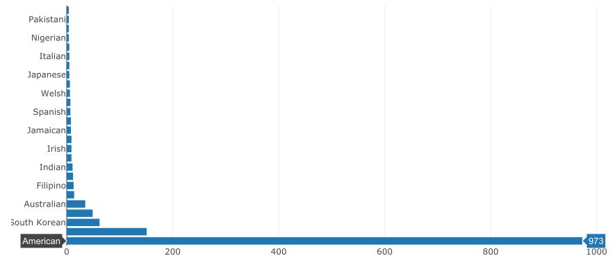
The result is quite coherent with the previous one. Being American should help once again.
What kind of music should you play?
For this question, we relied on Google Trends and extracted a CSV file over the past 5 years comparing the research interest in the most popular music styles.
genres = pd.read_csv('genres.csv', skiprows=1)
genres.plot(figsize=(15,10))
plt.show()
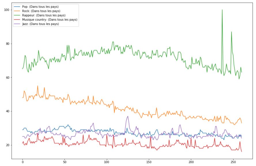
Rap music has over the past years invaded the music industry, and Google Trends reflects it pretty well.
**Conclusion **: This is all for the first part of this Hackathon story. If you liked it, please check the second part!